Home / Physical Chemistry · Electrochemistry / Class 6
Class 06 · 19 September 2026

Ion–Dipole & Ion–Quadrupole Interactions — Multipole Derivations & 23 Solved Problems

Class 5 finished electrode kinetics; Class 6 goes back to the solution side and asks the most basic question of all: what does an ion actually feel? Starting from Coulomb's law and nothing else, the lecture builds the multipole expansion step by step — first an ion plus a dipole, then an ion plus a planar quadrupole — and then spends the rest of the class turning those results (and the Born equation) into 23 fully worked numericals: solvation energies, Ka from concentrations and conductivities, angle and distance scaling of the multipole energies.

Semester VII Physical Chemistry Electrochemistry 15 source pages ≈ 25 min read
2master derivations (multipole)
3distance laws: 1/r, 1/r², 1/r³
23solved problems
2animated labs
Unit 4 · Electrochemistry III Live

00 Overview

Class 6 — lecture of 19 Sep 2026, fifteen scanned pages in two booklets — is a two-act class. Act I (four derivation pages) starts from Coulomb's law and nothing else, and builds the multipole expansion: the exact electrostatic potential of an ion sitting near a dipole, expanded term by term until the clean 1/R31/R^3 ion–dipole law drops out — then the same machinery applied to a planar quadrupole. Act II (eleven problem pages) is a pure problem set: twenty-three worked numericals on Born solvation, ion–dipole and ion–quadrupole energies, solvation thermodynamics, and ion-association constants.

The lecture in three laws

Uii∝1/rU_{ii} \propto 1/r — ion–ion, Coulomb's law (Sections 7).
Uid∝1/r2U_{id} \propto 1/r^2 — ion–dipole, Sections 1–2.
Uiq∝1/r3U_{iq} \propto 1/r^3 — ion–quadrupole, Sections 3–5.
Each extra multipole order costs one more power of distance — that is the whole moral of the multipole expansion, and Section 12 tables it.

  • Sections 1–2 + lab derive the ion–dipole potential ψ=2qzd/R3\psi = 2qzd/R^3 and the interaction energy U=Zie⋅2qzd/R3U = Z_i e \cdot 2qzd/R^3.
  • Sections 3–5 derive the ion–quadrupole potential and U=−Zie0μD/r2+2Zie0q(α2−β2)/r3U = -Z_i e_0 \mu_D/r^2 + 2Z_i e_0 q(\alpha^2-\beta^2)/r^3.
  • Sections 6–12 the lecture's own twenty-three solved problems, worked in full.
  • Sections 13–17 equation sheet, symbol table, rapid revision, editor's notes, raw scans.

01 Ion–dipole interaction: the geometry

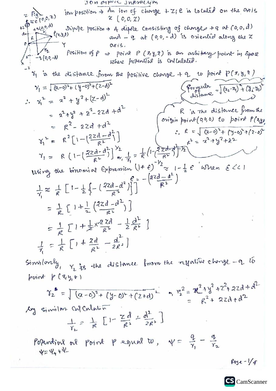
Put an ion of charge +Zie+Z_i e on the zz-axis at (0,0,z)(0, 0, z), and a dipole along the same axis: charge +q+q at (0,0,d)(0, 0, d) and charge −q-q at (0,0,−d)(0, 0, -d). The potential at an arbitrary point P(x,y,z)P(x, y, z) is the sum of the two Coulomb terms — and the entire derivation is just careful bookkeeping of the two distances.

z x y O +Zᵢe +q −q d d P r₁ r₂ R
Fig 1. The ion–dipole geometry (notebook p. 1/4): ion +Zie+Z_i e on the zz-axis, dipole ±q\pm q at ±d\pm d along the same axis, field point P(x,y,z)P(x,y,z) with distances r1r_1, r2r_2 and RR.

The distance from the positive charge to PP:

ir1=(x−0)2+(y−0)2+(z−d)2r_1 = \sqrt{(x-0)^2 + (y-0)^2 + (z-d)^2}
iir12=x2+y2+(z−d)2=x2+y2+z2−2zd+d2=R2−2zd+d2\begin{aligned} r_1^2 &= x^2 + y^2 + (z-d)^2 \\ &= x^2 + y^2 + z^2 - 2zd + d^2 \\ &= R^2 - 2zd + d^2 \end{aligned}

where R=x2+y2+z2R = \sqrt{x^2+y^2+z^2} is the distance from the origin to PP (margin note). Factoring out R2R^2:

iiir12=R2[1−2zd−d2R2],r1=R(1−2zd−d2R2)1/2r_1^2 = R^2\left[1 - \frac{2zd - d^2}{R^2}\right], \qquad r_1 = R\left(1 - \frac{2zd - d^2}{R^2}\right)^{1/2}
iv1r1=1R(1−2zd−d2R2)−1/2\frac{1}{r_1} = \frac{1}{R}\left(1 - \frac{2zd - d^2}{R^2}\right)^{-1/2}

Now the binomial expansion (1+ε)−1/2≈1−12ε(1+\varepsilon)^{-1/2} \approx 1 - \tfrac{1}{2}\varepsilon for ε≪1\varepsilon \ll 1, with ε=−(2zd−d2)/R2\varepsilon = -(2zd-d^2)/R^2:

v1r1≈1R[1−12{−(2zd−d2R2)}]=1R[1+12(2zd−d2R2)]\frac{1}{r_1} \approx \frac{1}{R}\left[1 - \frac{1}{2}\left\{-\left(\frac{2zd - d^2}{R^2}\right)\right\}\right] = \frac{1}{R}\left[1 + \frac{1}{2}\left(\frac{2zd - d^2}{R^2}\right)\right]
vi1r1=1R[1+zdR2−d22R2]\frac{1}{r_1} = \frac{1}{R}\left[1 + \frac{zd}{R^2} - \frac{d^2}{2R^2}\right]

Similarly for the negative charge, r22=x2+y2+z2+2zd+d2=R2+2zd+d2r_2^2 = x^2 + y^2 + z^2 + 2zd + d^2 = R^2 + 2zd + d^2, and by the same calculation:

vii1r2=1R[1−zdR2−d22R2]\frac{1}{r_2} = \frac{1}{R}\left[1 - \frac{zd}{R^2} - \frac{d^2}{2R^2}\right]
What just happened

Nothing physical yet — only geometry plus the binomial theorem. The two expansions differ only in the sign of the zd/R2zd/R^2 term. That sign difference is the entire dipole: when the two Coulomb potentials are subtracted, everything else cancels and the dipole moment survives. Section 2 does the subtraction.

02 Ion–dipole potential and interaction energy

The potential at PP is the sum of the two charge contributions, ψ=ψ++ψ−=q/r1−q/r2\psi = \psi_+ + \psi_- = q/r_1 - q/r_2:

viiiψ=q(1r1−1r2)\psi = q\left(\frac{1}{r_1} - \frac{1}{r_2}\right)
ixψ=qR{1+zdR2−d22R2−1+zdR2+d22R2}=qR⋅2zdR2\psi = \frac{q}{R}\left\{1 + \frac{zd}{R^2} - \frac{d^2}{2R^2} - 1 + \frac{zd}{R^2} + \frac{d^2}{2R^2}\right\} = \frac{q}{R}\cdot\frac{2zd}{R^2}

The constant and d2d^2 terms cancel (crossed out in the notebook), leaving the boxed dipole potential:

xψ=2qzdR3\psi = \frac{2qzd}{R^3}

The interaction energy of the ion ZieZ_i e in this potential is U=Zie ψU = Z_i e\,\psi:

xiU=Zie 2qzdR3=Zie 2qzd(x2+y2+z2)3/2valid for R≫dU = Z_i e\,\frac{2qzd}{R^3} = \frac{Z_i e\, 2qzd}{(x^2+y^2+z^2)^{3/2}} \qquad \text{valid for } R \gg d
Read the result

The potential of a dipole falls as 1/R31/R^3 — one power faster than a bare charge — and the interaction energy carries the dipole's charge separation 2qd2qd explicitly. The condition R≫dR \gg d is where the binomial expansion was legal: the field point must be far compared with the dipole's own size.

⊕ Lab · the dipole's orientation

The lecture gave you the sign of the answer — angle 0° = attraction, 180° = repulsion — but not the feeling of it. Spin the water molecules yourself: a lone Na⁺ has no chemistry of its own, yet it rotates five polar molecules into a hydration shell. Each oxygen points its negative end at the ion; flip the field and the molecules flip with it.

visual lab 1

Watch water pick a side

One ion, six water molecules. Flip the charge and watch every dipole re-aim itself — this lock-in is the ion–dipole interaction of Section 1.

δ−δ+δ−δ+δ−δ+δ−δ+δ−δ+δ−δ++
orientation: O ends (δ−) face the ion

Amber = O (δ−), cyan = H (δ+). The alignment is electrostatic and permanent on average — that ordering of solvent is exactly why ΔSsolv < 0 (Section 7) and why the Eley–Evans inner term is negative (Class 2, Section 5).

03 Ion–quadrupole interaction: the setup

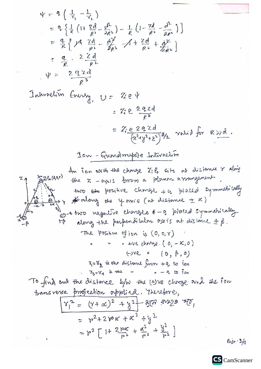
Now the dipole is replaced by a planar quadrupole: two positive charges +q+q placed symmetrically at ±α\pm\alpha along the yy-axis, and two negative charges −q-q at ±β\pm\beta along the perpendicular axis. An ion of charge Zie0Z_i e_0 sits on the zz-axis at (0,0,r)(0, 0, r). By symmetry r1=r2r_1 = r_2 (ion to the two +q+q charges) and r3=r4r_3 = r_4 (ion to the two −q-q charges) — so only two distances need expanding.

z y x O Zᵢe₀ +q +q α −q −q β r₁ r₂ r₃
Fig 2. The ion–quadrupole geometry (notebook p. 2/4): ion Zie0Z_i e_0 at (0,0,r)(0,0,r) above a planar charge arrangement — +q+q at ±α\pm\alpha on one axis, −q−q at ±β\pm\beta on the perpendicular axis.

The notebook finds the distances by a "transverse projection" construction (boxed in the original):

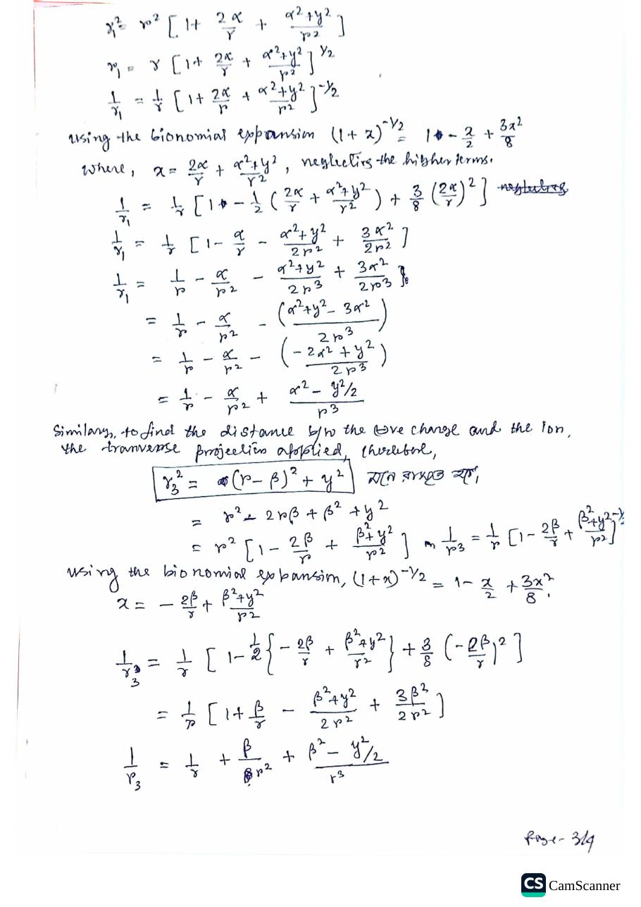
xiir12=(r+α)2+y2=r2+2rα+α2+y2=r2[1+2αr+α2+y2r2]r_1^2 = (r + \alpha)^2 + y^2 = r^2 + 2r\alpha + \alpha^2 + y^2 = r^2\left[1 + \frac{2\alpha}{r} + \frac{\alpha^2 + y^2}{r^2}\right]
xiiir32=(r−β)2+y2=r2−2rβ+β2+y2=r2[1−2βr+β2+y2r2]r_3^2 = (r - \beta)^2 + y^2 = r^2 - 2r\beta + \beta^2 + y^2 = r^2\left[1 - \frac{2\beta}{r} + \frac{\beta^2 + y^2}{r^2}\right]

04 Expanding 1/r11/r_1 and 1/r31/r_3

The quadrupole needs one more order than the dipole did: the expansion of (1+x)−1/2=1−x/2+3x2/8(1+x)^{-1/2} = 1 - x/2 + 3x^2/8 is carried to the 1/r31/r^3 term, higher terms neglected.

xiv1r1=1r[1+2αr+α2+y2r2]−1/2\frac{1}{r_1} = \frac{1}{r}\left[1 + \frac{2\alpha}{r} + \frac{\alpha^2 + y^2}{r^2}\right]^{-1/2}

With x=2α/r+(α2+y2)/r2x = 2\alpha/r + (\alpha^2+y^2)/r^2:

xv1r1=1r[1−12(2αr+α2+y2r2)+38(2αr)2]\frac{1}{r_1} = \frac{1}{r}\left[1 - \frac{1}{2}\left(\frac{2\alpha}{r} + \frac{\alpha^2 + y^2}{r^2}\right) + \frac{3}{8}\left(\frac{2\alpha}{r}\right)^2\right]
xvi1r1=1r−αr2+α2−y2/2r3\frac{1}{r_1} = \frac{1}{r} - \frac{\alpha}{r^2} + \frac{\alpha^2 - y^2/2}{r^3}

The notebook shows the intermediate algebra: 1/r−α/r2−(α2+y2)/2r3+3α2/2r31/r - \alpha/r^2 - (\alpha^2+y^2)/2r^3 + 3\alpha^2/2r^3, which collects to the form above. Similarly, with x=−2β/r+(β2+y2)/r2x = -2\beta/r + (\beta^2+y^2)/r^2:

xvii1r3=1r[1−12{−2βr+β2+y2r2}+38(−2βr)2]=1r[1+βr−β2+y22r2+3β22r2]\frac{1}{r_3} = \frac{1}{r}\left[1 - \frac{1}{2}\left\{-\frac{2\beta}{r} + \frac{\beta^2 + y^2}{r^2}\right\} + \frac{3}{8}\left(-\frac{2\beta}{r}\right)^2\right] = \frac{1}{r}\left[1 + \frac{\beta}{r} - \frac{\beta^2 + y^2}{2r^2} + \frac{3\beta^2}{2r^2}\right]
xviii1r3=1r+βr2+β2−y2/2r3\frac{1}{r_3} = \frac{1}{r} + \frac{\beta}{r^2} + \frac{\beta^2 - y^2/2}{r^3}

05 Quadrupole potential and interaction energy

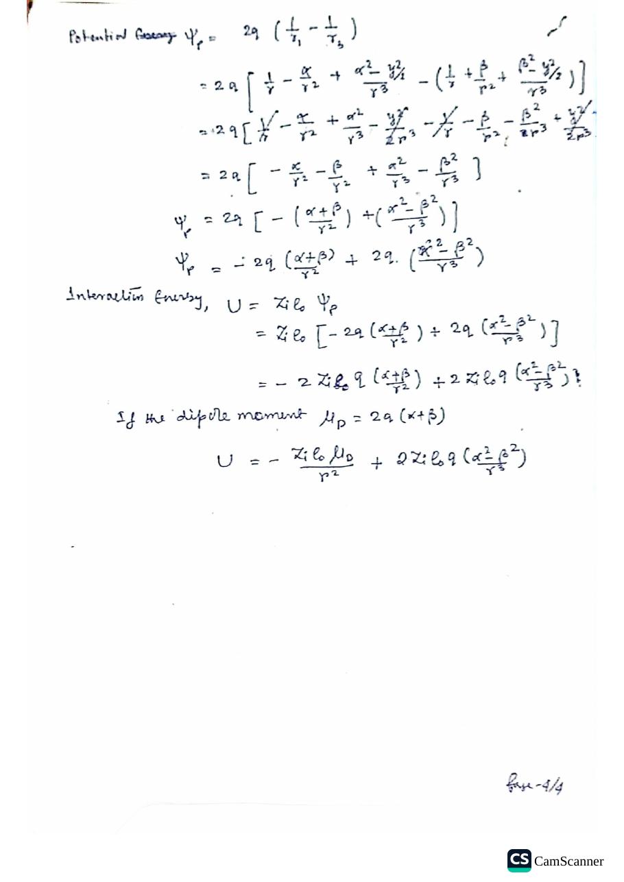
Two +q+q charges at distance r1r_1 and two −q−q at r3r_3 give the potential ψp=2q(1/r1−1/r3)\psi_p = 2q(1/r_1 - 1/r_3) (the notes call this "potential energy" ψp\psi_p; the interaction energy follows as U=Zie0ψpU = Z_i e_0\psi_p):

xixψp=2q[1r−αr2+α2−y2/2r3−(1r+βr2+β2−y2/2r3)]\psi_p = 2q\left[\frac{1}{r} - \frac{\alpha}{r^2} + \frac{\alpha^2 - y^2/2}{r^3} - \left(\frac{1}{r} + \frac{\beta}{r^2} + \frac{\beta^2 - y^2/2}{r^3}\right)\right]

The 1/r1/r and y2y^2 terms cancel (crossed out in the notebook):

xxψp=2q[−α+βr2+α2−β2r3]=−2q(α+βr2)+2q(α2−β2r3)\psi_p = 2q\left[-\frac{\alpha + \beta}{r^2} + \frac{\alpha^2 - \beta^2}{r^3}\right] = -2q\left(\frac{\alpha + \beta}{r^2}\right) + 2q\left(\frac{\alpha^2 - \beta^2}{r^3}\right)

Multiplying by the ion charge Zie0Z_i e_0 and writing the dipole moment μD=2q(α+β)\mu_D = 2q(\alpha+\beta):

xxiU=−Zie0 μDr2+2Zie0q(α2−β2r3)U = -\frac{Z_i e_0\,\mu_D}{r^2} + 2Z_i e_0 q\left(\frac{\alpha^2 - \beta^2}{r^3}\right)
Why two terms survive

A quadrupole is the next multipole after the dipole, and its potential properly falls as 1/r31/r^3 — but this planar charge arrangement also carries a net dipole moment μD\mu_D, whose 1/r21/r^2 contribution dominates at large rr. The pure quadrupole piece is the second term, proportional to the asymmetry α2−β2\alpha^2-\beta^2.

06 The lecture's solved problems — Born solvation (1–4)

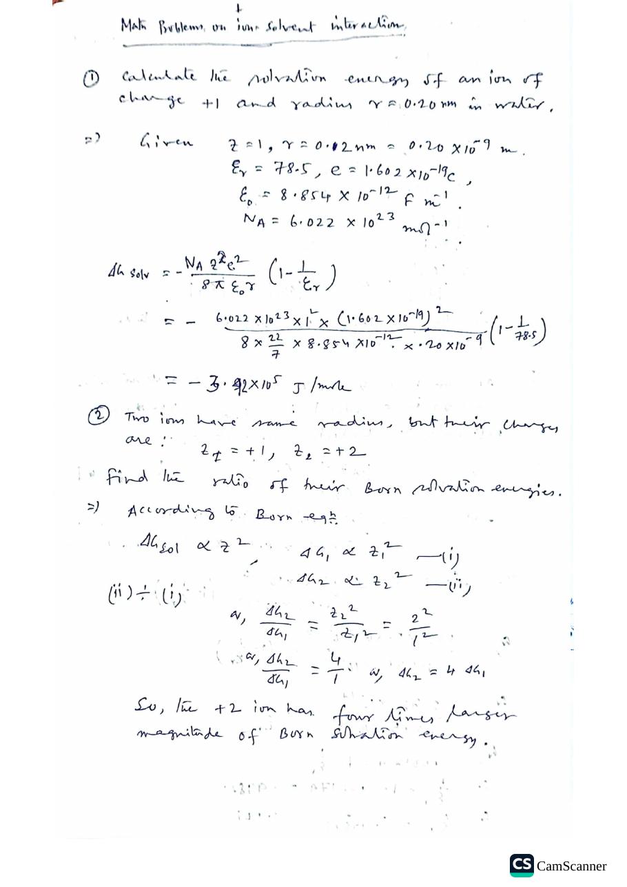
The second booklet is a pure problem set. Reproduced in full, arithmetic checked. Constants used throughout: e=1.602×10⁻¹⁹ Ce = 1.602\times10^{-19}\ \text{C}, ε0=8.854×10⁻¹² F m−1\varepsilon_0 = 8.854\times10^{-12}\ \text{F m}^{-1}, NA=6.022×10²³ mol−1N_A = 6.022\times10^{23}\ \text{mol}^{-1}.

Solv. 1Born equation · numerical

Q. Calculate the solvation energy of an ion of charge +1 and radius r=0.20 nmr = 0.20\ \text{nm} in water (εr=78.5\varepsilon_r = 78.5).

Ans. Given z=1z = 1, r=0.20×10⁻⁹ mr = 0.20\times10^{-9}\ \text{m}. The molar Born equation:

ΔGsolv=−NAz2e28πε0r(1−1εr)\Delta G_{\text{solv}} = -\frac{N_A z^2 e^2}{8\pi\varepsilon_0 r}\left(1 - \frac{1}{\varepsilon_r}\right)
=−6.022×1023×12×(1.602×10−19)28×227×8.854×10−12×0.20×10−9(1−178.5)=−3.42×10⁵ J mol−1= -\frac{6.022\times10^{23}\times 1^2\times(1.602\times10^{-19})^2}{8\times\frac{22}{7}\times 8.854\times10^{-12}\times 0.20\times10^{-9}}\left(1 - \frac{1}{78.5}\right) = -3.42\times10^5\ \text{J mol}^{-1}
Solv. 2Born equation · ratio

Q. Two ions have the same radius, but charges z1=+1z_1 = +1, z2=+2z_2 = +2. Find the ratio of their Born solvation energies.

Ans. ΔGsol∝z2\Delta G_{\text{sol}} \propto z^2, so ΔG1∝z12\Delta G_1 \propto z_1^2 and ΔG2∝z22\Delta G_2 \propto z_2^2:

ΔG2ΔG1=z22z12=2212=41⇒ΔG2=4ΔG1\frac{\Delta G_2}{\Delta G_1} = \frac{z_2^2}{z_1^2} = \frac{2^2}{1^2} = \frac{4}{1} \quad\Rightarrow\quad \Delta G_2 = 4\Delta G_1

The +2 ion has four times the magnitude of Born solvation energy.

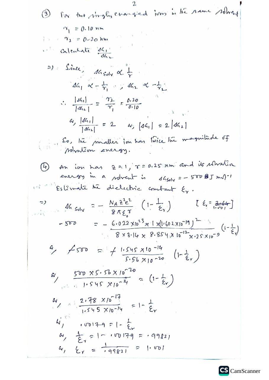
Solv. 3Born equation · ratio

Q. For two singly charged ions in the same solvent: r1=0.10 nmr_1 = 0.10\ \text{nm}, r2=0.20 nmr_2 = 0.20\ \text{nm}. Calculate ΔG1/ΔG2\Delta G_1/\Delta G_2.

Ans. ΔGsolv∝1/r\Delta G_{\text{solv}} \propto 1/r:

∣ΔG1∣∣ΔG2∣=r2r1=0.200.10=2⇒∣ΔG1∣=2∣ΔG2∣\frac{|\Delta G_1|}{|\Delta G_2|} = \frac{r_2}{r_1} = \frac{0.20}{0.10} = 2 \quad\Rightarrow\quad |\Delta G_1| = 2|\Delta G_2|

The smaller ion has twice the magnitude of solvation energy.

Solv. 4Born equation · invert for ε

Q. An ion has z=1z = 1, r=0.25 nmr = 0.25\ \text{nm} and its solvation energy in a solvent is ΔGsolv=−500 J mol−1\Delta G_{\text{solv}} = -500\ \text{J mol}^{-1}. Estimate the dielectric constant εr\varepsilon_r.

Ans.

−500=−6.022×1023×1×(1.602×10−19)28×3.14×8.854×10−12×0.25×10−9(1−1εr)-500 = -\frac{6.022\times10^{23}\times 1\times(1.602\times10^{-19})^2}{8\times 3.14\times 8.854\times10^{-12}\times 0.25\times10^{-9}}\left(1 - \frac{1}{\varepsilon_r}\right)
500=1.545×10−145.56×10⁻²⁰(1−1εr)  ⇒  0.00179=1−1εr500 = \frac{1.545\times10^{-14}}{5.56\times10^{-20}}\left(1 - \frac{1}{\varepsilon_r}\right) \;\Rightarrow\; 0.00179 = 1 - \frac{1}{\varepsilon_r}
1εr=0.99821⇒εr=1.001\frac{1}{\varepsilon_r} = 0.99821 \quad\Rightarrow\quad \varepsilon_r = 1.001

A barely-polar solvent: with εr ≈ 1 there is almost no dielectric stabilisation, so even a modest |ΔG| forces εr down to ~1.

07 Solved problems — ion–ion & ion–dipole energy (5–6)

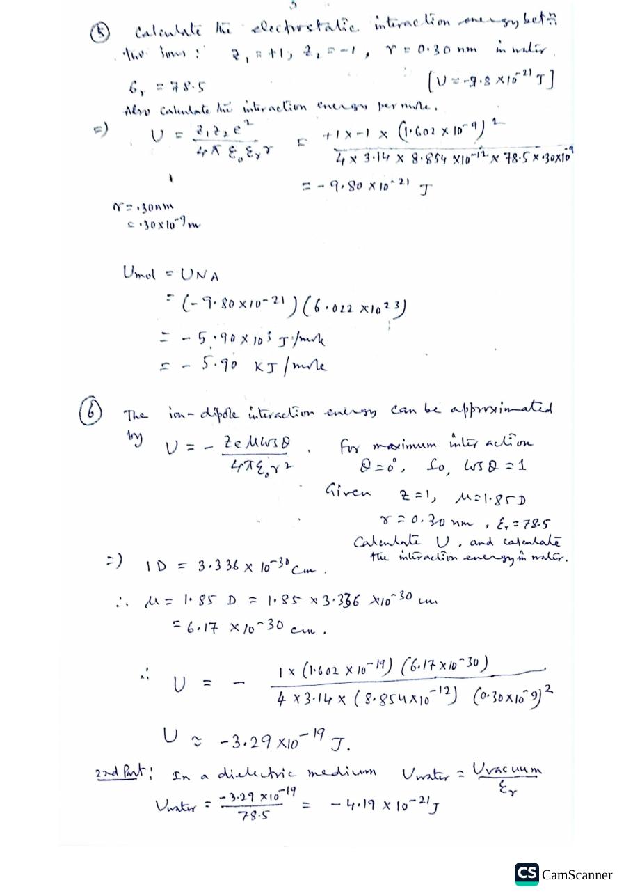
Solv. 5ion–ion energy · per mole

Q. Calculate the electrostatic interaction energy between two ions z1=+1z_1 = +1, z2=−1z_2 = -1, r=0.30 nmr = 0.30\ \text{nm} in water (εr=78.5\varepsilon_r = 78.5), and the interaction energy per mole.

Ans.

U=z1z2e24πε0εrr=(+1×−1)×(1.602×10−19)24×3.14×8.854×10−12×78.5×0.30×10−9=−9.80×10⁻²¹ JU = \frac{z_1 z_2 e^2}{4\pi\varepsilon_0\varepsilon_r r} = \frac{(+1\times-1)\times(1.602\times10^{-19})^2}{4\times 3.14\times 8.854\times10^{-12}\times 78.5\times 0.30\times10^{-9}} = -9.80\times10^{-21}\ \text{J}
Umol=UNA=(−9.80×10⁻²¹)(6.022×10²³)=−5.90×10³ J mol−1=−5.90 kJ mol−1U_{\text{mol}} = UN_A = (-9.80\times10^{-21})(6.022\times10^{23}) = -5.90\times10^3\ \text{J mol}^{-1} = -5.90\ \text{kJ mol}^{-1}
Solv. 6ion–dipole energy · vacuum vs water

Q. The ion–dipole energy is U=−zeμcos⁡θ/4πε0r2U = -ze\mu\cos\theta/4\pi\varepsilon_0 r^2. For maximum interaction θ=0∘\theta = 0^\circ (cos⁡θ=1\cos\theta = 1). Given z=1z = 1, μ=1.85 D\mu = 1.85\ \text{D}, r=0.30 nmr = 0.30\ \text{nm}, εr=78.5\varepsilon_r = 78.5: calculate UU, and the interaction energy in water.

Ans. 1 D=3.336×10⁻³⁰ C m1\ \text{D} = 3.336\times10^{-30}\ \text{C m}, so μ=1.85×3.336×10−30=6.17×10⁻³⁰ C m\mu = 1.85\times 3.336\times10^{-30} = 6.17\times10^{-30}\ \text{C m}:

U=−1×(1.602×10−19)(6.17×10⁻³⁰)4×3.14×(8.854×10−12)(0.30×10⁻⁹)2≈−3.29×10⁻¹⁹ JU = -\frac{1\times(1.602\times10^{-19})(6.17\times10^{-30})}{4\times 3.14\times(8.854\times10^{-12})(0.30\times10^{-9})^2} \approx -3.29\times10^{-19}\ \text{J}

In a dielectric medium Uwater=Uvacuum/εrU_{\text{water}} = U_{\text{vacuum}}/\varepsilon_r:

Uwater=−3.29×10−1978.5=−4.19×10⁻²¹ JU_{\text{water}} = \frac{-3.29\times10^{-19}}{78.5} = -4.19\times10^{-21}\ \text{J}

08 Solved problems — solvation thermodynamics & hydration number (7–8)

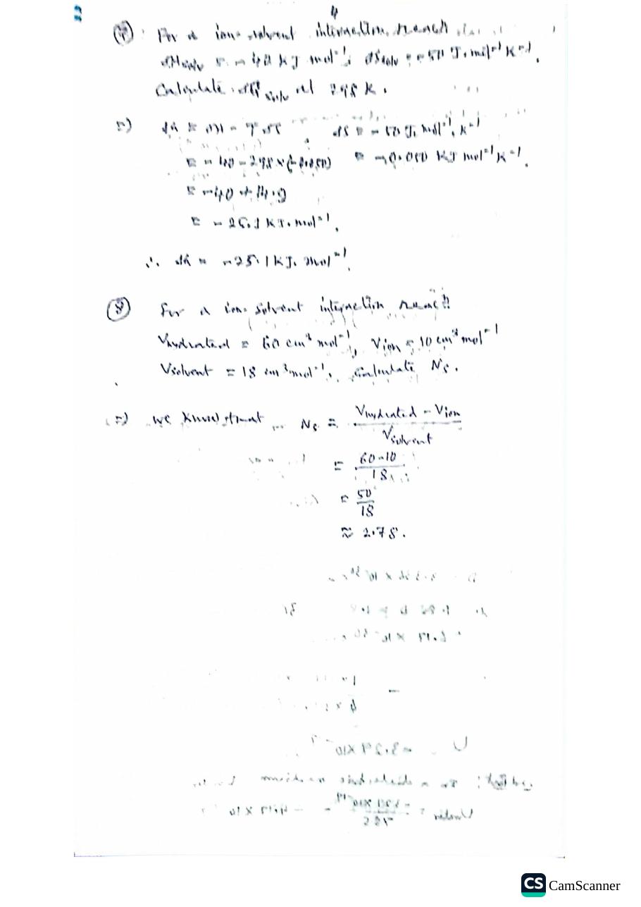
Solv. 7ΔG from ΔH, ΔS

Q. For an ion–solvent interaction, ΔHsolv=−42 kJ mol−1\Delta H_{\text{solv}} = -42\ \text{kJ mol}^{-1}; ΔSsolv=−50 J mol−1K−1\Delta S_{\text{solv}} = -50\ \text{J mol}^{-1}\text{K}^{-1}. Calculate ΔGsolv\Delta G_{\text{solv}} at 298 K.

Ans. ΔG=ΔH−TΔS\Delta G = \Delta H - T\Delta S, with ΔS=−0.050 kJ mol−1K−1\Delta S = -0.050\ \text{kJ mol}^{-1}\text{K}^{-1}:

ΔG=−42−298×(−0.050)=−42+14.9=−26.1 kJ mol−1\Delta G = -42 - 298\times(-0.050) = -42 + 14.9 = -26.1\ \text{kJ mol}^{-1}
Solv. 8hydration number

Q. For an ion–solvent interaction: Vhydrated=60 cm3mol−1V_{\text{hydrated}} = 60\ \text{cm}^3\text{mol}^{-1}, Vion=10 cm3mol−1V_{\text{ion}} = 10\ \text{cm}^3\text{mol}^{-1}, Vsolvent=18 cm3mol−1V_{\text{solvent}} = 18\ \text{cm}^3\text{mol}^{-1}. Calculate NsN_s.

Ans. Ns=(Vhydrated−Vion)/VsolventN_s = (V_{\text{hydrated}} - V_{\text{ion}})/V_{\text{solvent}}:

Ns=60−1018=5018≈2.78N_s = \frac{60 - 10}{18} = \frac{50}{18} \approx 2.78

09 Solved problems — ion association & Ka (1–8)

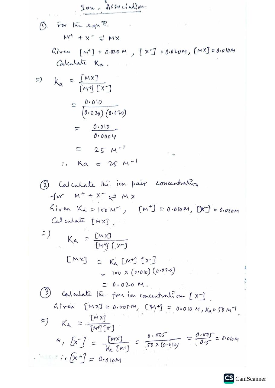
For the equilibrium M++X−⇌MXM^+ + X^- \rightleftharpoons MX, Ka=[MX]/[M+][X−]K_a = [MX]/[M^+][X^-]. For a 1:1 electrolyte of total concentration CC with fraction dissociated α\alpha: Ka=(1−α)/Cα2K_a = (1-\alpha)/C\alpha^2.

Assoc. 1Ka from concentrations

Q. For M++X−⇌MXM^+ + X^- \rightleftharpoons MX: [M+]=0.020 M[M^+] = 0.020\ \text{M}, [X−]=0.020 M[X^-] = 0.020\ \text{M}, [MX]=0.010 M[MX] = 0.010\ \text{M}. Calculate KaK_a.

Ka=[MX][M+][X−]=0.010(0.020)(0.020)=0.0100.0004=25 M−1K_a = \frac{[MX]}{[M^+][X^-]} = \frac{0.010}{(0.020)(0.020)} = \frac{0.010}{0.0004} = 25\ \text{M}^{-1}
Assoc. 2ion-pair concentration

Q. Ka=100 M−1K_a = 100\ \text{M}^{-1}, [M+]=0.010 M[M^+] = 0.010\ \text{M}, [X−]=0.020 M[X^-] = 0.020\ \text{M}. Calculate [MX][MX].

[MX]=Ka[M+][X−]=100×(0.010)(0.020)=0.020 M[MX] = K_a[M^+][X^-] = 100\times(0.010)(0.020) = 0.020\ \text{M}
Assoc. 3free-ion concentration

Q. [MX]=0.005 M[MX] = 0.005\ \text{M}, [M+]=0.010 M[M^+] = 0.010\ \text{M}, Ka=50 M−1K_a = 50\ \text{M}^{-1}. Calculate the free ion concentration [X−][X^-].

[X−]=[MX]Ka[M+]=0.00550×0.010=0.0050.5=0.010 M[X^-] = \frac{[MX]}{K_a[M^+]} = \frac{0.005}{50\times 0.010} = \frac{0.005}{0.5} = 0.010\ \text{M}
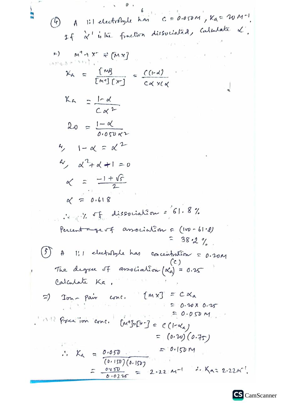
Assoc. 4α from Ka · quadratic

Q. A 1:1 electrolyte has C=0.050 MC = 0.050\ \text{M}, Ka=20 M−1K_a = 20\ \text{M}^{-1}. If α\alpha is the fraction dissociated, calculate α\alpha.

Ka=[MX][M+][X−]=C(1−α)Cα⋅Cα=1−αCα2K_a = \frac{[MX]}{[M^+][X^-]} = \frac{C(1-\alpha)}{C\alpha\cdot C\alpha} = \frac{1-\alpha}{C\alpha^2}
20=1−α0.050 α2  ⇒  1−α=α2  ⇒  α2+α−1=020 = \frac{1-\alpha}{0.050\,\alpha^2} \;\Rightarrow\; 1-\alpha = \alpha^2 \;\Rightarrow\; \alpha^2 + \alpha - 1 = 0
α=−1+52=0.618\alpha = \frac{-1 + \sqrt{5}}{2} = 0.618

Percentage dissociation = 61.8%; percentage association = 38.2%.

Assoc. 5Ka from degree of association

Q. A 1:1 electrolyte has concentration C=0.20 MC = 0.20\ \text{M}. The degree of association αa=0.25\alpha_a = 0.25. Calculate KaK_a.

Ans. Ion-pair conc. [MX]=Cαa=0.20×0.25=0.050 M[MX] = C\alpha_a = 0.20\times0.25 = 0.050\ \text{M}; free ion conc. [M+]=[X−]=C(1−αa)=0.150 M[M^+] = [X^-] = C(1-\alpha_a) = 0.150\ \text{M}:

Ka=0.050(0.150)(0.150)=0.0500.0225=2.22 M−1K_a = \frac{0.050}{(0.150)(0.150)} = \frac{0.050}{0.0225} = 2.22\ \text{M}^{-1}
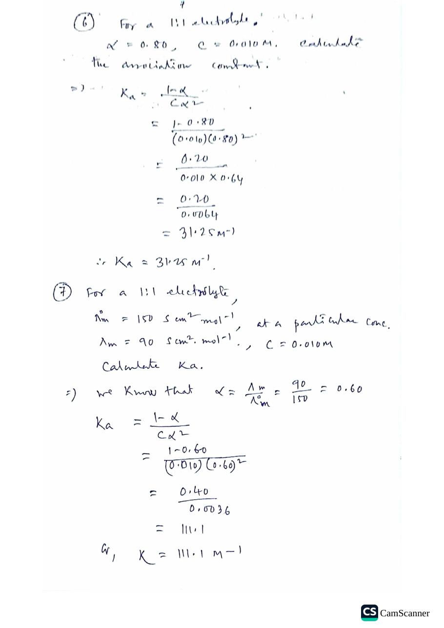
Assoc. 6Ka from α

Q. For a 1:1 electrolyte, α=0.80\alpha = 0.80, C=0.010 MC = 0.010\ \text{M}. Calculate the association constant.

Ka=1−αCα2=1−0.80(0.010)(0.80)2=0.200.0064=31.25 M−1K_a = \frac{1-\alpha}{C\alpha^2} = \frac{1-0.80}{(0.010)(0.80)^2} = \frac{0.20}{0.0064} = 31.25\ \text{M}^{-1}
Assoc. 7α from conductivity → Ka

Q. For a 1:1 electrolyte, Λm∘=150 S cm2mol−1\Lambda_m^\circ = 150\ \text{S cm}^2\text{mol}^{-1}; at a particular concentration Λm=90 S cm2mol−1\Lambda_m = 90\ \text{S cm}^2\text{mol}^{-1}, C=0.010 MC = 0.010\ \text{M}. Calculate KaK_a.

Ans. α=Λm/Λm∘=90/150=0.60\alpha = \Lambda_m/\Lambda_m^\circ = 90/150 = 0.60:

Ka=1−αCα2=0.40(0.010)(0.60)2=0.400.0036=111.1 M−1K_a = \frac{1-\alpha}{C\alpha^2} = \frac{0.40}{(0.010)(0.60)^2} = \frac{0.40}{0.0036} = 111.1\ \text{M}^{-1}
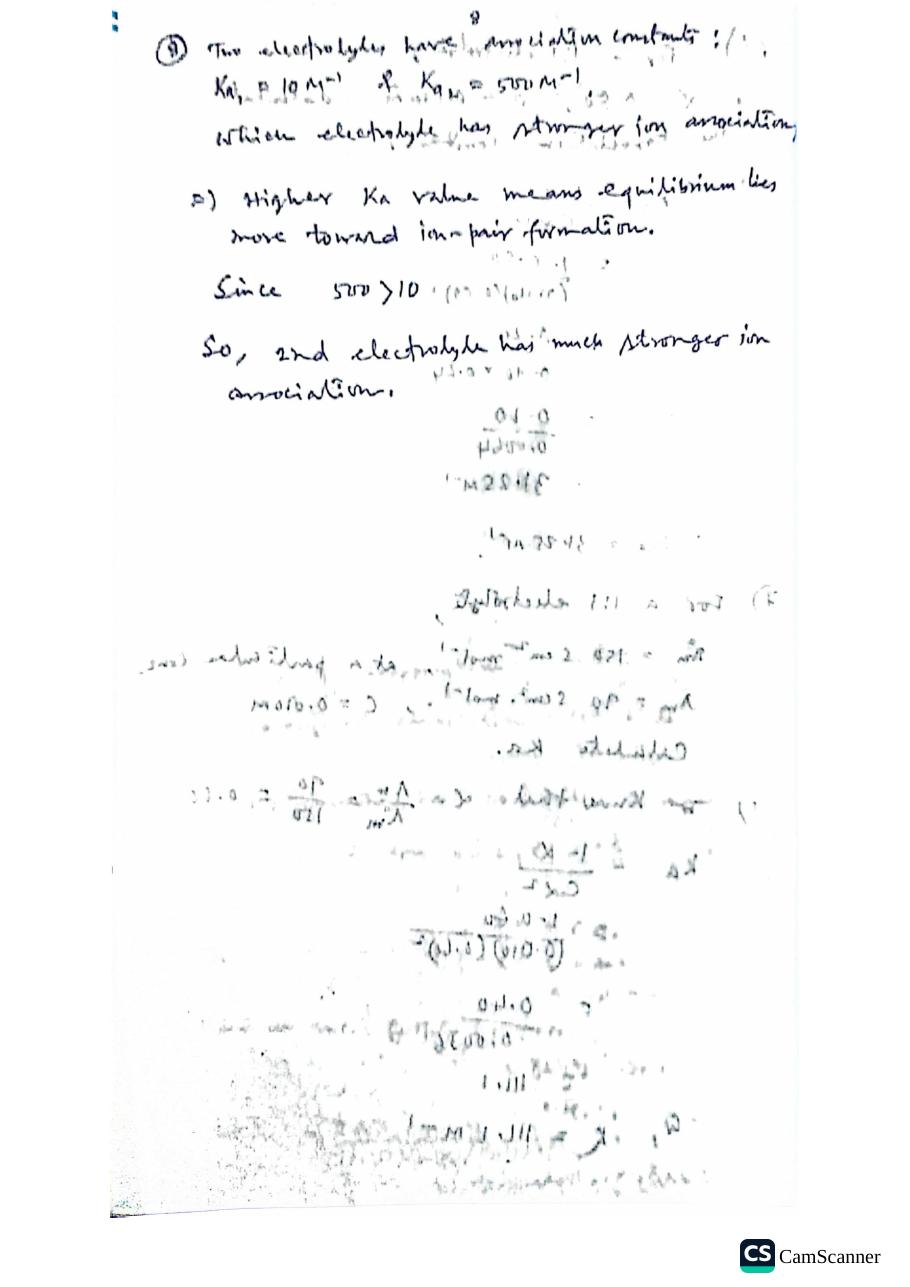
Assoc. 8comparing association strength

Q. Two electrolytes have association constants Ka1=10 M−1K_{a1} = 10\ \text{M}^{-1} and Ka2=500 M−1K_{a2} = 500\ \text{M}^{-1}. Which has stronger ion association?

Ans. A higher KaK_a means the equilibrium lies further toward ion-pair formation. Since 500 > 10, the second electrolyte has much stronger ion association.

⊕ Lab · the pairing window

Eight association problems computed Kₐ for fixed constants — this lab answers the prior question: when should ions pair at all? Bjerrum's length is the distance where the Coulomb energy equals k_BT; below it, the electrostatic pull beats thermal motion and ion pairs win. Push the dielectric up to 78.5 and watch the pairing window collapse — that is why water dissociates salts.

visual lab 7

How wide is the pairing window?

The green band is the association region a ≤ r ≤ r_B drawn to scale. Cool the solution, drop the dielectric constant, or raise the charge product — and watch the window open.

04812162024r (Å)a = 3.0rB = 7.14 År < a: impossibleion pairfree ions →
r(B) = 7.14 Å pairing window = 4.14 Å r(B) ∝ 1/T, 1/ε(r), |z+ z−|

Sanity value: water (ε = 78.5) at 298 K, 1:1 electrolyte → r(B) ≈ 7.1 Å, the textbook number. Wider window = more separations count as associated = larger K(A) (Sections 7–8).

10 Solved problems — ion–dipole angle & distance (1–3)

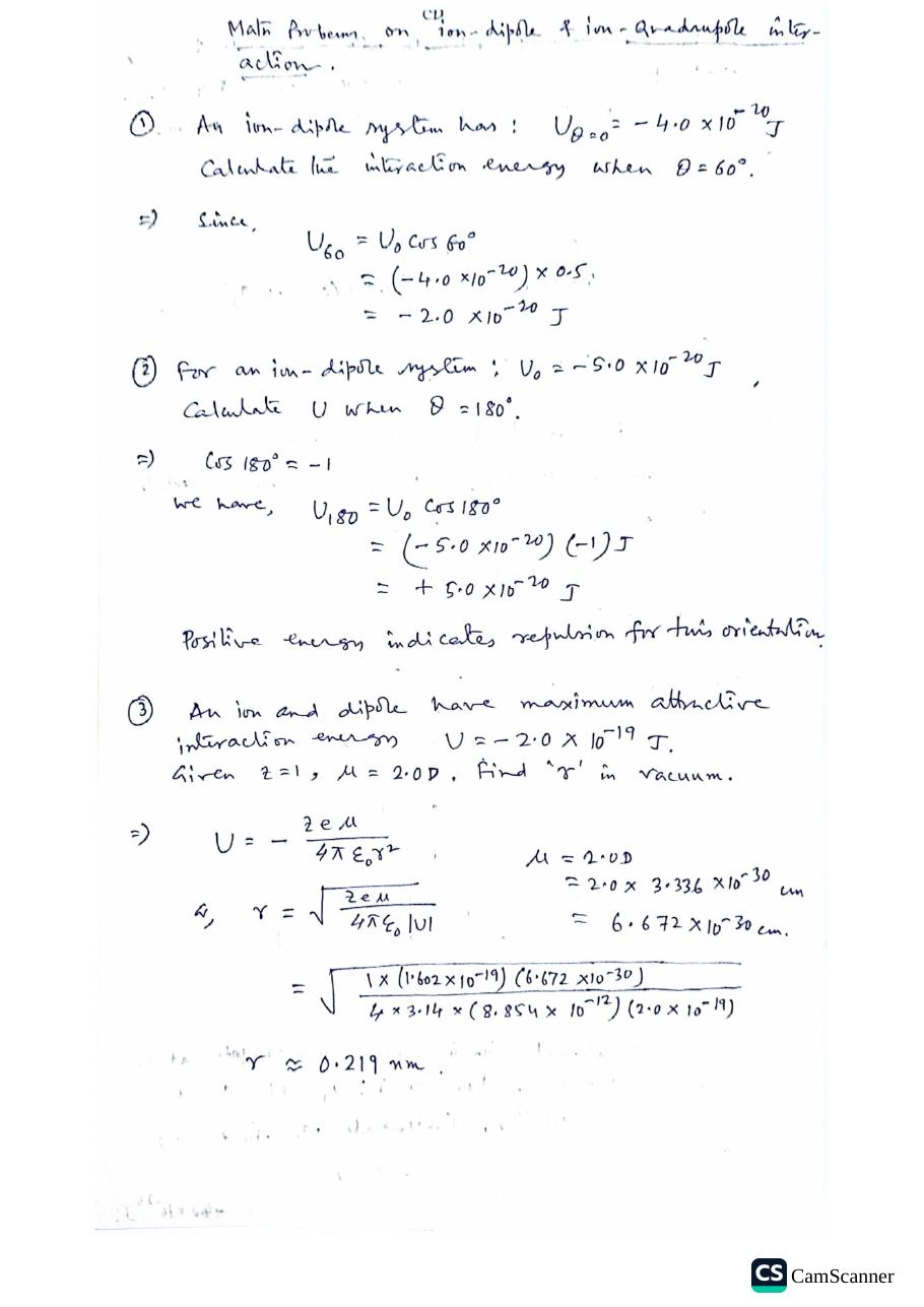
M.P. 1U(θ) = U₀cosθ

Q. An ion–dipole system has Uθ=0=−4.0×10⁻²⁰ JU_{\theta=0} = -4.0\times10^{-20}\ \text{J}. Calculate the interaction energy when θ=60∘\theta = 60^\circ.

U60=U0cos⁡60∘=(−4.0×10−20)×0.5=−2.0×10⁻²⁰ JU_{60} = U_0\cos 60^\circ = (-4.0\times10^{-20})\times 0.5 = -2.0\times10^{-20}\ \text{J}
M.P. 2θ = 180° · repulsion

Q. For an ion–dipole system: U0=−5.0×10⁻²⁰ JU_0 = -5.0\times10^{-20}\ \text{J}. Calculate UU when θ=180∘\theta = 180^\circ.

U180=U0cos⁡180∘=(−5.0×10⁻²⁰)(−1)=+5.0×10⁻²⁰ JU_{180} = U_0\cos 180^\circ = (-5.0\times10^{-20})(-1) = +5.0\times10^{-20}\ \text{J}

Positive energy indicates repulsion for this orientation.

M.P. 3invert U for r

Q. An ion and dipole have maximum attractive interaction energy U=−2.0×10⁻¹⁹ JU = -2.0\times10^{-19}\ \text{J}. Given z=1z = 1, μ=2.0 D\mu = 2.0\ \text{D}. Find rr in vacuum.

Ans. U=−zeμ/4πε0r2U = -ze\mu/4\pi\varepsilon_0 r^2, so r=zeμ/4πε0∣U∣r = \sqrt{ze\mu/4\pi\varepsilon_0|U|}; μ=2.0×3.336×10−30=6.672×10⁻³⁰ C m\mu = 2.0\times 3.336\times10^{-30} = 6.672\times10^{-30}\ \text{C m}:

r=1×(1.602×10−19)(6.672×10⁻³⁰)4×3.14×(8.854×10−12)(2.0×10⁻¹⁹)≈0.219 nmr = \sqrt{\frac{1\times(1.602\times10^{-19})(6.672\times10^{-30})}{4\times 3.14\times(8.854\times10^{-12})(2.0\times10^{-19})}} \approx 0.219\ \text{nm}

11 Solved problems — ion–quadrupole (4–6)

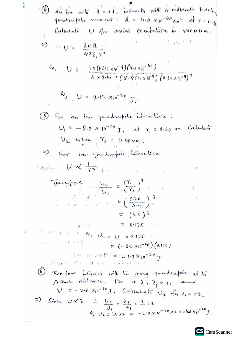
M.P. 4U = zeQ/4πε₀r³

Q. An ion with z=+1z = +1 interacts with a molecule having quadrupole moment Q=4.0×10−40 C m2Q = 4.0\times10^{-40}\ \text{C m}^2 at r=0.30 nmr = 0.30\ \text{nm}. Calculate UU for axial orientation in vacuum.

U=zeQ4πε0r3=1×(1.602×10−19)(4.0×10−40)4×3.14×(8.854×10−12)(0.30×10⁻⁹)3=2.13×10⁻²⁰ JU = \frac{zeQ}{4\pi\varepsilon_0 r^3} = \frac{1\times(1.602\times10^{-19})(4.0\times10^{-40})}{4\times 3.14\times(8.854\times10^{-12})(0.30\times10^{-9})^3} = 2.13\times10^{-20}\ \text{J}
M.P. 5U ∝ 1/r³ scaling

Q. For an ion–quadrupole interaction: U1=−8.0×10⁻²⁰ JU_1 = -8.0\times10^{-20}\ \text{J} at r1=0.20 nmr_1 = 0.20\ \text{nm}. Calculate U2U_2 when r2=0.40 nmr_2 = 0.40\ \text{nm}.

Ans. U∝1/r3U \propto 1/r^3:

U2U1=(r1r2)3=(0.200.40)3=0.125\frac{U_2}{U_1} = \left(\frac{r_1}{r_2}\right)^3 = \left(\frac{0.20}{0.40}\right)^3 = 0.125
U2=(−8.0×10−20)×0.125=−1.0×10⁻²⁰ JU_2 = (-8.0\times10^{-20})\times 0.125 = -1.0\times10^{-20}\ \text{J}
M.P. 6U ∝ z scaling

Q. Two ions interact with the same quadrupole at the same distance. Ion 1: z1=+1z_1 = +1, U1=−2.0×10⁻²⁰ JU_1 = -2.0\times10^{-20}\ \text{J}. Calculate U2U_2 for z2=+2z_2 = +2.

Ans. U∝zU \propto z:

U2U1=z2z1=2⇒U2=−4.0×10⁻²⁰ J\frac{U_2}{U_1} = \frac{z_2}{z_1} = 2 \quad\Rightarrow\quad U_2 = -4.0\times10^{-20}\ \text{J}

12 How the interaction energy changes with distance

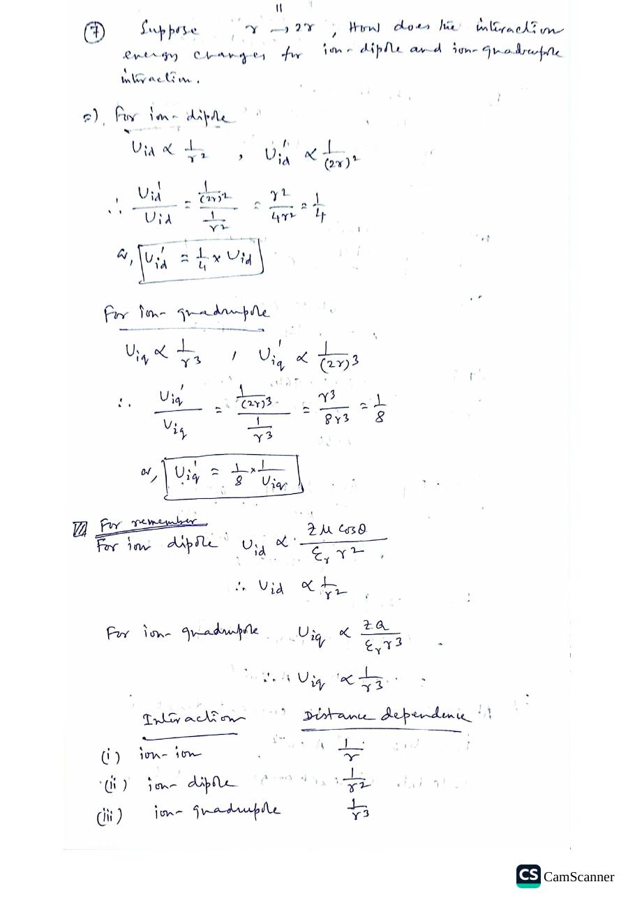
M.P. 7r → 2r scaling

Q. Suppose r→2rr \to 2r. How does the interaction energy change for ion–dipole and ion–quadrupole interaction?

Ans. For ion–dipole, Uid∝1/r2U_{id} \propto 1/r^2:

Uid′Uid=1/(2r)21/r2=14⇒Uid′=14Uid\frac{U_{id}'}{U_{id}} = \frac{1/(2r)^2}{1/r^2} = \frac{1}{4} \quad\Rightarrow\quad \boxed{U_{id}' = \tfrac{1}{4}U_{id}}

For ion–quadrupole, Uiq∝1/r3U_{iq} \propto 1/r^3:

Uiq′Uiq=1/(2r)31/r3=18⇒Uiq′=18Uiq\frac{U_{iq}'}{U_{iq}} = \frac{1/(2r)^3}{1/r^3} = \frac{1}{8} \quad\Rightarrow\quad \boxed{U_{iq}' = \tfrac{1}{8}U_{iq}}
For remember (boxed in the notebook)

For ion–dipole Uid∝zμcos⁡θ/εrr2U_{id} \propto z\mu\cos\theta/\varepsilon_r r^2, hence Uid∝1/r2U_{id} \propto 1/r^2.
For ion–quadrupole Uiq∝zQ/εrr3U_{iq} \propto zQ/\varepsilon_r r^3, hence Uiq∝1/r3U_{iq} \propto 1/r^3.

InteractionDistance dependence
(i) ion–ion1/r1/r
(ii) ion–dipole1/r21/r^2
(iii) ion–quadrupole1/r31/r^3
10 0 10 1 10 2 r / r₀ 10 −7 10 −6 10 −5 10 −4 10 −3 10 −2 10 −1 10 0 |U| / U₀ ion–ion ∝ 1/r ion–dipole ∝ 1/r² ion–quadrupole ∝ 1/r³
Fig 3. How fast each interaction dies with distance — log–log plot of |U|/U₀ against r/r₀: ion–ion ∝ 1/r, ion–dipole ∝ 1/r², ion–quadrupole ∝ 1/r³ (the notebook's "for remember" box, drawn).

13 The equation sheet, at a glance

Every boxed result of the lecture on one screen; labels match the sections above.

xψ=2qzdR3\psi = \dfrac{2qzd}{R^3}
xiU=Zie 2qzdR3(R≫d)U = \dfrac{Z_i e\, 2qzd}{R^3} \quad (R \gg d)
xxiU=−Zie0 μDr2+2Zie0qα2−β2r3U = -\dfrac{Z_i e_0\,\mu_D}{r^2} + 2Z_i e_0 q\dfrac{\alpha^2 - \beta^2}{r^3}
BΔGsolv=−NAz2e28πε0r(1−1εr)\Delta G_{\text{solv}} = -\dfrac{N_A z^2 e^2}{8\pi\varepsilon_0 r}\left(1 - \dfrac{1}{\varepsilon_r}\right)
KKa=[MX][M+][X−]=1−αCα2K_a = \dfrac{[MX]}{[M^+][X^-]} = \dfrac{1-\alpha}{C\alpha^2}
θU(θ)=U0cos⁡θ,U=−zeμcos⁡θ4πε0r2U(\theta) = U_0\cos\theta, \qquad U = -\dfrac{ze\mu\cos\theta}{4\pi\varepsilon_0 r^2}
QU=zeQ4πε0r3U = \dfrac{zeQ}{4\pi\varepsilon_0 r^3}
rUii∝1r,Uid∝1r2,Uiq∝1r3U_{ii}\propto\tfrac{1}{r}, \quad U_{id}\propto\tfrac{1}{r^2}, \quad U_{iq}\propto\tfrac{1}{r^3}

14 Symbol table

SymbolMeaningFirst seen
ZieZ_i echarge of the ion (+Zie)§1
±q, d\pm q,\ ddipole charges and half-separation§1
P(x,y,z), RP(x,y,z),\ Rfield point; distance OP§1
r1, r2r_1,\ r_2distances +q→P, −q→P§1
ψ\psielectrostatic potential§2
UUinteraction energy§2
α, β\alpha,\ \betaquadrupole half-separations (+q, −q)§3
r3r_3distance −q→ion§3
ψp\psi_pquadrupole potential§5
μD\mu_Ddipole moment, 2q(α+β)2q(\alpha+\beta)§5
μ\mumolecular dipole moment (problems)§7
QQquadrupole moment (problems)§11
KaK_aion-association constant§9
α\alphafraction dissociated§9
NsN_shydration (solvation) number§8
Λm\Lambda_mmolar conductivity§9

15 Rapid revision

  • The whole derivation is geometry + binomial expansion: write 1/r11/r_1 and 1/r21/r_2 as series in the small ratio (dipole size)/(field distance), subtract — only the dipole term survives.
  • Ion–dipole: ψ=2qzd/R3\psi = 2qzd/R^3, U=Zie⋅2qzd/R3U = Z_i e\cdot 2qzd/R^3, valid for R≫dR \gg d.
  • Ion–quadrupole: expand one order further (1/r31/r^3); U=−Zie0μD/r2+2Zie0q(α2−β2)/r3U = -Z_i e_0\mu_D/r^2 + 2Z_i e_0 q(\alpha^2-\beta^2)/r^3.
  • Distance ladder: ion–ion 1/r1/r → ion–dipole 1/r21/r^2 → ion–quadrupole 1/r31/r^3 — each multipole order costs one power of rr.
  • Born: ΔGsolv∝z2/r\Delta G_{\text{solv}} \propto z^2/r — charge matters as the square, size inversely.
  • Association: Ka=[MX]/[M+][X−]=(1−α)/Cα2K_a = [MX]/[M^+][X^-] = (1-\alpha)/C\alpha^2; conductivity gives α=Λm/Λm∘\alpha = \Lambda_m/\Lambda_m^\circ.
  • Orientation: U(θ)=U0cos⁡θU(\theta) = U_0\cos\theta — maximum attraction at θ=0∘\theta = 0^\circ, repulsion at 180∘180^\circ.
  • Doubling the distance quarters an ion–dipole energy and eighths an ion–quadrupole energy.

16 Editor's notes

Uncertainties flagged in the transcription, resolved with chemistry sense — nothing else was changed.

  • Heading reconstruction: the top heading of derivation page 1 is cropped at the scan edge ("Ion Dipole Interac…"); restored as "Ion–Dipole Interaction" from the visible remainder and content.
  • Charge exponent: the elementary charge was written as (1.602×10⁻⁹)2(1.602\times10^{-9})^2 in Solv. 5; corrected to 10−1910^{-19} — the value e=1.602×10⁻¹⁹ Ce = 1.602\times10^{-19}\ \text{C} is stated explicitly on the first problem page and the worked answer requires it.
  • Illegible glyph: an unreadable symbol between "−500" and "J mol⁻¹" in Solv. 4 was dropped; the calculation is unaffected.
  • Illegible salt name: the compound name before ΔHsolv in Solv. 7 could not be read; the problem is stated for a generic ion–solvent interaction.
  • Inferred unit: the distance in M.P. 4 is cut off at the page edge ("r = 0.3…"); nm was inferred from the worked calculation (0.30×10⁻⁹)3(0.30\times10^{-9})^3.
  • Quadratic sign: in Assoc. 4 the sign before the 1 in α2+α−1=0\alpha^2+\alpha-1 = 0 looks corrected in the handwriting; the algebra and the stated root α=(−1+5)/2\alpha = (-1+\sqrt5)/2 confirm it.
  • Notation kept as written: the notes use ψ\psi for the electrostatic potential and call ψp=2q(1/r1−1/r3)\psi_p = 2q(1/r_1-1/r_3) the "potential energy"; transcribed verbatim.

17 Original notebook scans

Digitised from the class notebook of 19 Sep 2026 — two CamScanner booklets: four derivation pages (S1–S4, scanned 00:17) and eleven problem pages (S5–S15, scanned 00:22). Every equation above was cross-checked against these pages, and every numerical re-computed. Tap any thumbnail to open the full scan.