Class 04 · Factors of Ion Association & Electrode Kinetics

00 Overview

Class 3 ended with Bjerrum's machine: a distance $r_B$ , an integral $K_A$ , and an associated fraction $\alpha$ wired to conductivity. Class 4 — notebook pages 34–39, lecture of 05 Sep 2026 — turns the machine's dials one by one: which properties of the solvent, the ions and the solution push association up or down? Six factors, each with a proportionality the notebook writes out ( $K_A \propto 1/\varepsilon_r$ , $K_A \propto |z_+z_-|$ , $K_A \propto 1/T$ , plus size, concentration and polarizing power). Then the lecture spends the association it has built: ion pairs are neutral, neutral things carry no current, so every factor that raises association lowers conductivity — quantified by $\alpha = \Lambda_m/\Lambda_m^{\circ}$ .

Two movements, one lecture

Movement 1 (Sections 1–8): the six factors responsible for ion association, each with the notebook's proportionality and a snapshot figure. Movement 2 (Sections 9–11): the conductivity bill — free ions are the only charge carriers, so $\Lambda_m = \alpha\,\Lambda_m^{\circ}$ and the Λ-vs-c curve sinks below Λ°. Coda (Sections 12–15): a new topic — electrode kinetics: the current through an electrode is a direct readout of the electrode reaction rate, $I = nFv$ , with anode/cathode rates $I/2F$ and the limiting current at high concentration.

Section 1 recalls the ion-pair equilibrium and $K_A$ from Class 3.
Sections 2–7 walk the six factors: solvent dielectric, charge, size, concentration, temperature, polarizing power.
Section 8 + lab summarises them and lets you turn all six at once.
Sections 9–11 price association in conductivity: carriers, $\alpha = \Lambda_m/\Lambda_m^{\circ}$ , the Λ-vs-c gap.
Sections 12–15 + lab + calculator electrode kinetics: interface, $I = nFv$ , anode/cathode rates, I–v line and limiting current.
Sections 16–21 calculator, equation sheet, symbol table, rapid revision, raw scans, PYQ audit with worked examples.

01 The ion-pair equilibrium, recalled

In solution, oppositely charged ions associate to form ion pairs — the equilibrium Class 3 built and the notebook rewrites on page 34 as the starting point of this lecture:

\mathrm{A}^{2+} + \mathrm{B}^{2-} \rightleftharpoons \mathrm{AB} \quad (\text{ion pair})

The forward direction is association; its extent is governed by the association constant $K_A$ (Bjerrum's integral, Class 3 Section 7). Everything in Sections 2–7 is really a statement about what makes $K_A$ — and with it the paired fraction — grow or shrink.

Reading the proportionality signs

The notebook writes each factor as a proportionality of $K_A$ . Read " $K_A \propto 1/\varepsilon_r$ " as: everything else fixed, lowering the dielectric constant raises the association constant. These are ceteris-paribus arrows, not a single combined formula — the lab in Section 8 combines them only as a teaching snapshot.

02 Factor 1 — nature of the solvent (dielectric constant $\varepsilon_r$ )

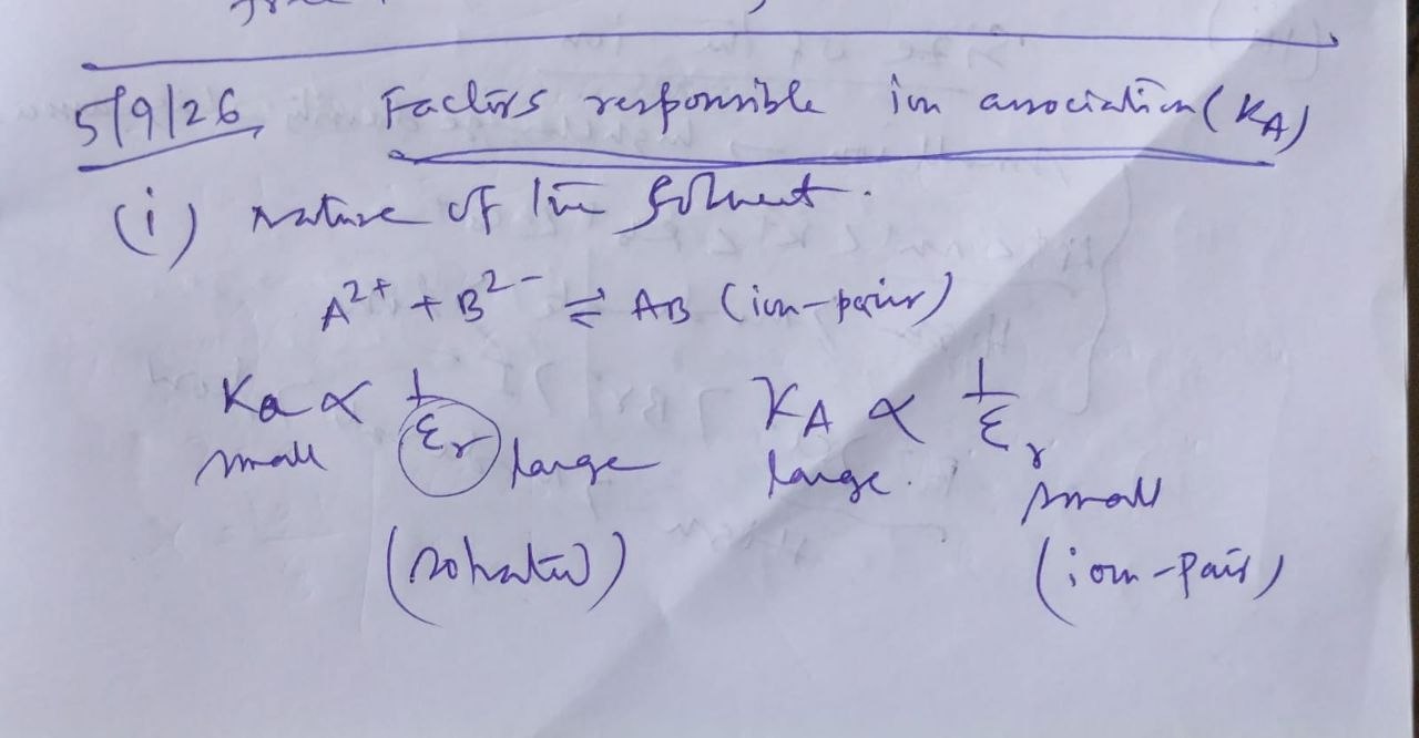
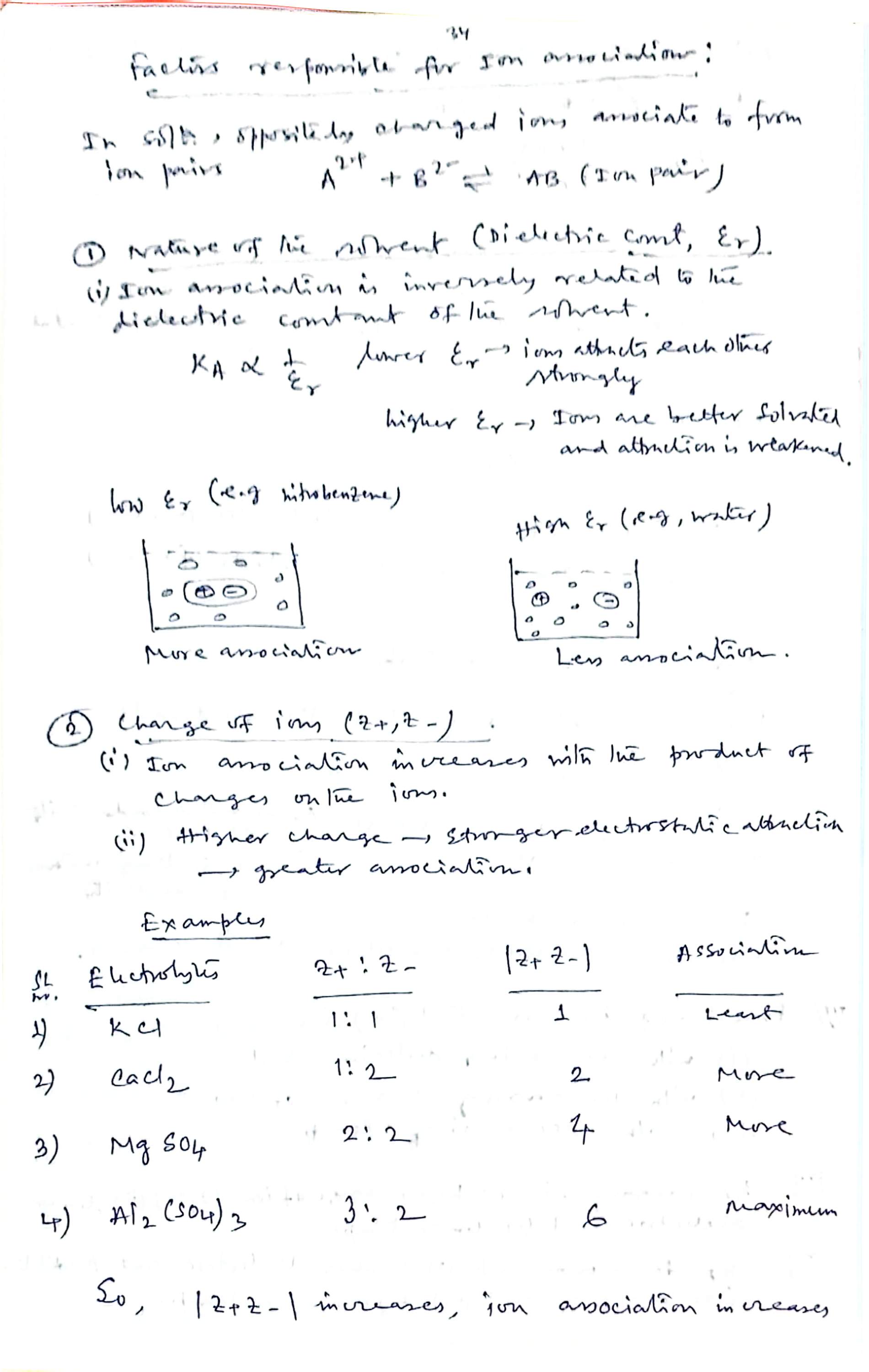
Ion association is inversely related to the dielectric constant of the solvent:

K_A \propto \frac{1}{\varepsilon_r}

Lower $\varepsilon_r$ → ions attract each other strongly. The solvent screens the Coulomb force weakly, so the pair holds together — more association.
Higher $\varepsilon_r$ → ions are better solvated and the attraction is weakened — less association.

The notebook's own contrast: low $\varepsilon_r$ (e.g. nitrobenzene) — the snapshot shows contact pairs; high $\varepsilon_r$ (e.g. water) — the snapshot shows separated, solvated ions.

Fig 1. Dielectric screening decides the pairing: in a low-ε(r) solvent (A, nitrobenzene ≈ 35) contact pairs survive; in a high-ε(r) solvent (B, water ≈ 78) solvated ions stay apart — K(A) ∝ 1/ε(r) (Section 2, notebook p34).

Why the screening works (Class 1 echo)

The Coulomb force between two charges in a medium is $F = q_1 q_2/(4\pi\varepsilon_0\varepsilon_r r^2)$ : $\varepsilon_r$ sits in the denominator. Water ( $\varepsilon_r \approx 78$ at 298 K) cuts the attraction to about a quarter of nitrobenzene's ( $\varepsilon_r \approx 35$ ) at the same distance — which is exactly the direction of $K_A \propto 1/\varepsilon_r$ . (Bjerrum's form of the same physics: $r_B \propto 1/\varepsilon_r$ , Class 3 Section 5.)

03 Factor 2 — charge on the ions ( $z_+, z_-$ )

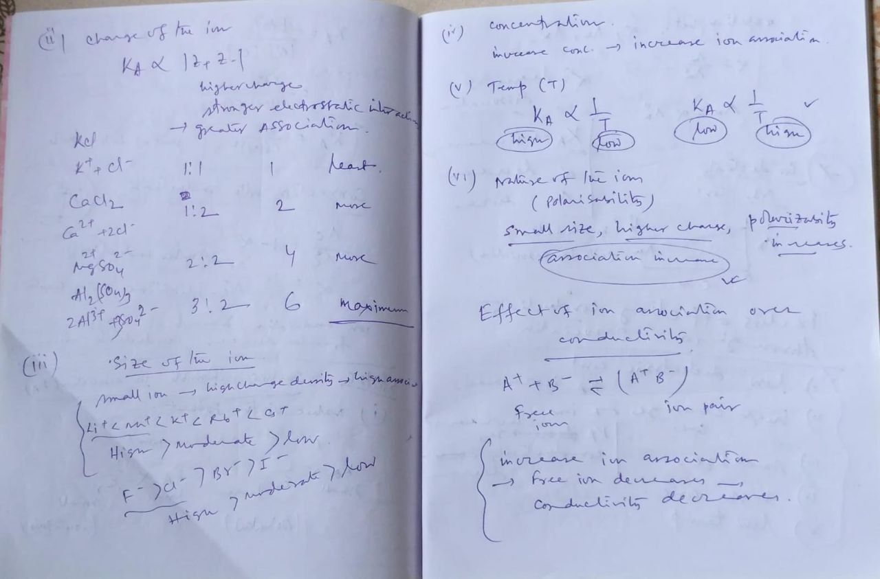
Ion association increases with the product of the charges on the ions:

iii

K_A \propto |z_+\,z_-|

Higher charge → stronger electrostatic attraction → greater association. The notebook proves the habit with a four-row ladder:

Sl. no.	Electrolyte	$z_+ : z_-$	$\|z_+ z_-\|$	Association
1	KCl ( $\mathrm{K}^+ + \mathrm{Cl}^-$ )	1 : 1	1	least
2	CaCl₂ ( $\mathrm{Ca}^{2+} + 2\,\mathrm{Cl}^-$ )	1 : 2	2	more
3	MgSO₄ ( $\mathrm{Mg}^{2+} + \mathrm{SO}_4^{2-}$ )	2 : 2	4	more
4	Al₂(SO₄)₃ ( $2\,\mathrm{Al}^{3+} + 3\,\mathrm{SO}_4^{2-}$ )	3 : 2	6	maximum

So, as $|z_+z_-|$ increases, ion association increases — multivalent salts pair hard.

Fig 2. The charge ladder of the notebook table: |z(+) z(−)| = 1, 2, 4, 6 for KCl, CaCl₂, MgSO₄, Al₂(SO₄)₃ — association least → maximum (Section 3, p34).

04 Factor 3 — size of the ions

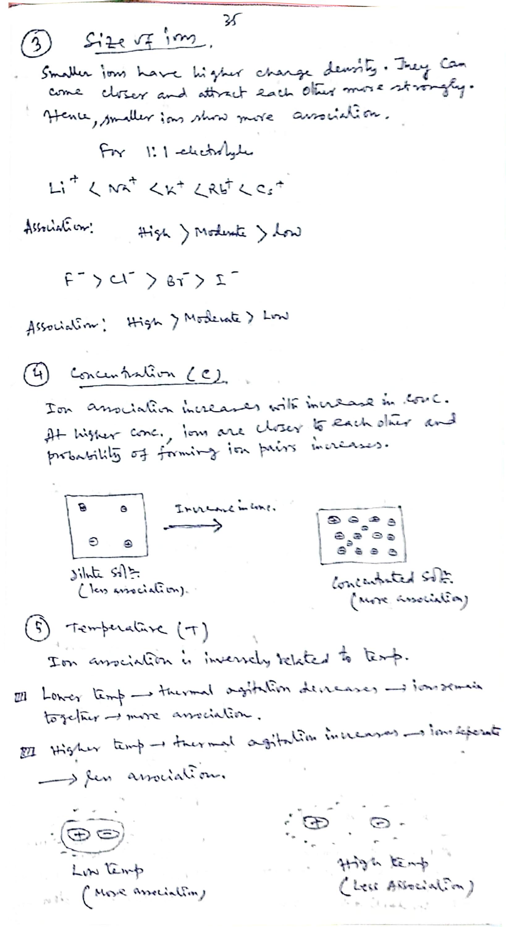
Smaller ions have higher charge density. They can come closer and attract each other more strongly. Hence, smaller ions show more association. For 1:1 electrolytes the notebook writes both series with the association trend beneath:

Cations: $\mathrm{Li}^+ < \mathrm{Na}^+ < \mathrm{K}^+ < \mathrm{Rb}^+ < \mathrm{Cs}^+$ in size, so association runs high > moderate > low along the series (Li⁺ pairs most, Cs⁺ least).
Anions: $\mathrm{F}^- > \mathrm{Cl}^- > \mathrm{Br}^- > \mathrm{I}^-$ in association — again high > moderate > low as the ion grows (F⁻ smallest, pairs most).

Fig 3. Size series at fixed 1:1 stoichiometry: association falls as the ion grows — Li⁺ → Cs⁺ and F⁻ → I⁻, high → moderate → low (Section 4, p35).

Same physics as Class 1, opposite costume

Charge density also drove the Born solvation energy ( $\Delta G \propto z^2/r$ ): small, highly charged ions grab solvent and counter-ions hardest. Here the grip is on the counter-ion; there it was on the dipoles. One inverse-distance law, two consequences.

05 Factor 4 — concentration ( $c$ )

Ion association increases with increase in concentration. At higher conc., ions are closer to each other and the probability of forming ion pairs increases. The notebook's two-box picture: a dilute solution with ions far apart (less association) becomes, on concentrating, a crowded box where contacts are frequent (more association).

Fig 4. Concentration snapshot: dilute (ions far apart, less association) versus concentrated (contacts frequent, more association) (Section 5, p35).

In Bjerrum's language this is bookkeeping rather than a change of $K_A$ itself: at higher $c$ the same equilibrium constant acts on larger ion densities, so the fraction paired rises — exactly the behaviour of $K_A = \alpha/[c(1-\alpha)^2]$ solved in Class 3 Section 10 (α → 0 only on dilution).

06 Factor 5 — temperature ( $T$ )

Ion association is inversely related to temperature:

K_A \propto \frac{1}{T}

Lower temp → thermal agitation decreases → ions remain together → more association ( $K_A$ high at low $T$ ).
Higher temp → thermal agitation increases → ions separate → less association ( $K_A$ low at high $T$ ).

Fig 5. Temperature: weak thermal agitation at low T lets the pair survive; strong agitation at high T knocks it apart — K(A) ∝ 1/T (Section 6, p35).

Bjerrum's equation carries the same arrow: $r_B = z_+z_-e^2/(4\pi\varepsilon_0\varepsilon_r k_BT) \propto 1/T$ — cooling widens the attraction-dominated window, so more pairs qualify as associated (Class 3, Prob. 1).

07 Factor 6 — nature of the ion (polarizing power)

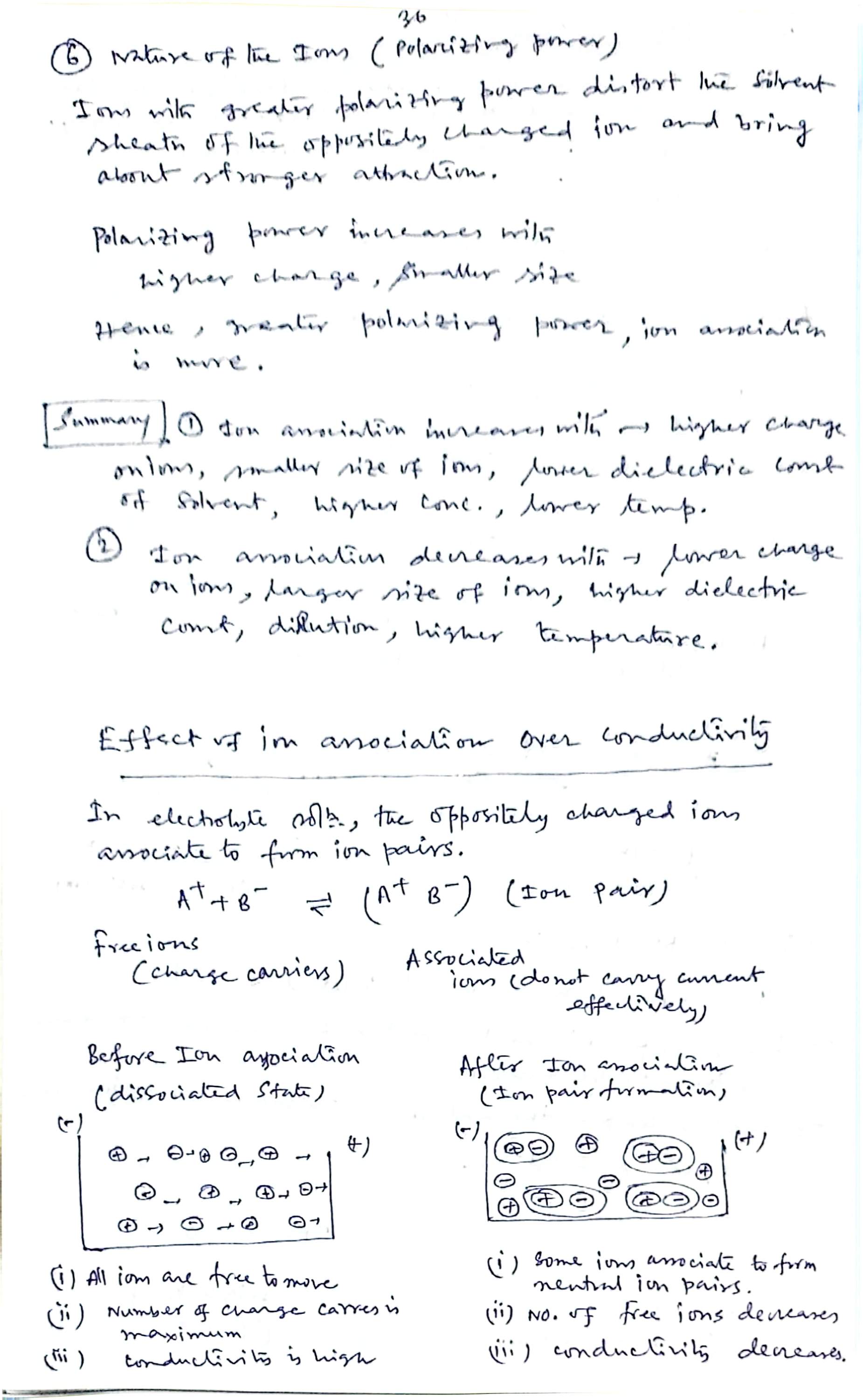
Ions with greater polarizing power distort the solvent sheath of the oppositely charged ion and bring about stronger attraction. Polarizing power increases with higher charge and smaller size — hence, greater polarizing power ⇒ more ion association.

The notebook's circle

Page 36 ends the factor list with the chain the lecture circled: small size, higher charge, polarizability increases ⇒ association increases. It is Factors 2 and 3 folded into one property: an ion that concentrates its charge (small, multivalent) polarises its partner's environment and pulls the pair together.

08 The six factors, summarised

Summary, as the notebook boxes it (p36)

(1) Association increases with → higher charge on ions, smaller size of ion, lower dielectric constant of solvent, higher concentration, lower temperature (and greater polarizing power).
(2) Association decreases with → lower charge on ions, larger size of ion, higher dielectric constant, dilution, higher temperature.

Five arrows, one mechanism: everything that strengthens the Coulomb grip relative to thermal agitation (charge, closeness, weak screening, cold) moves ions from the "free" column into the "paired" column. The lab below lets you turn all five dials at once and watch the snapshot re-sort itself.

visual lab 10

Turn the six factors

Five dials, one snapshot: the box holds twelve ions (six cation–anion couples). The lecture's five arrows (Sections 2–6) decide how many couples sit as contact pairs — low ε(r), high charge, small size, high concentration and low temperature all push ions into pairs; the opposites set them free.

Solvent ε(r) — 78

Concentration — 0.50 mol/L

Temperature — 298 K

Charge product |z+ z−|

Ion size

3/6 pairs · 6 free ions · association score 0.47 → moderate association

Illustrates Sections 2–8. The score blends the five dials with weights (0.24 ε(r), 0.24 charge, 0.18 size, 0.17 c, 0.17 T) so every arrow points the way the notebook's summary box does; it is a teaching snapshot, not a K(A) evaluation — for the quantitative machine see Class 3's Bjerrum calculator. Jiggle amplitude tracks T visually; under reduced motion the snapshot renders static with the same numbers.

09 What association costs conductivity

In electrolyte solution, the oppositely charged ions associate to form ion pairs:

\mathrm{A}^+ + \mathrm{B}^- \rightleftharpoons (\mathrm{A}^+\,\mathrm{B}^-) \quad (\text{ion pair})

The left-hand side are the free ions — the charge carriers; the right-hand side are associated ions, which do not carry current effectively. The notebook draws the cell before and after association:

Fig 6. The conductivity bill: before association every ion drifts in the field (carriers maximum); after association the neutral pairs sit out (carriers reduced, conductivity lower) (Section 9, p36).

Before association: (i) all ions are free to move; (ii) the number of charge carriers is maximum; (iii) conductivity is high.
After association: (i) some ions associate to form neutral ion pairs; (ii) the number of free ions decreases; (iii) conductivity decreases.

Reason, in three lines (p37)

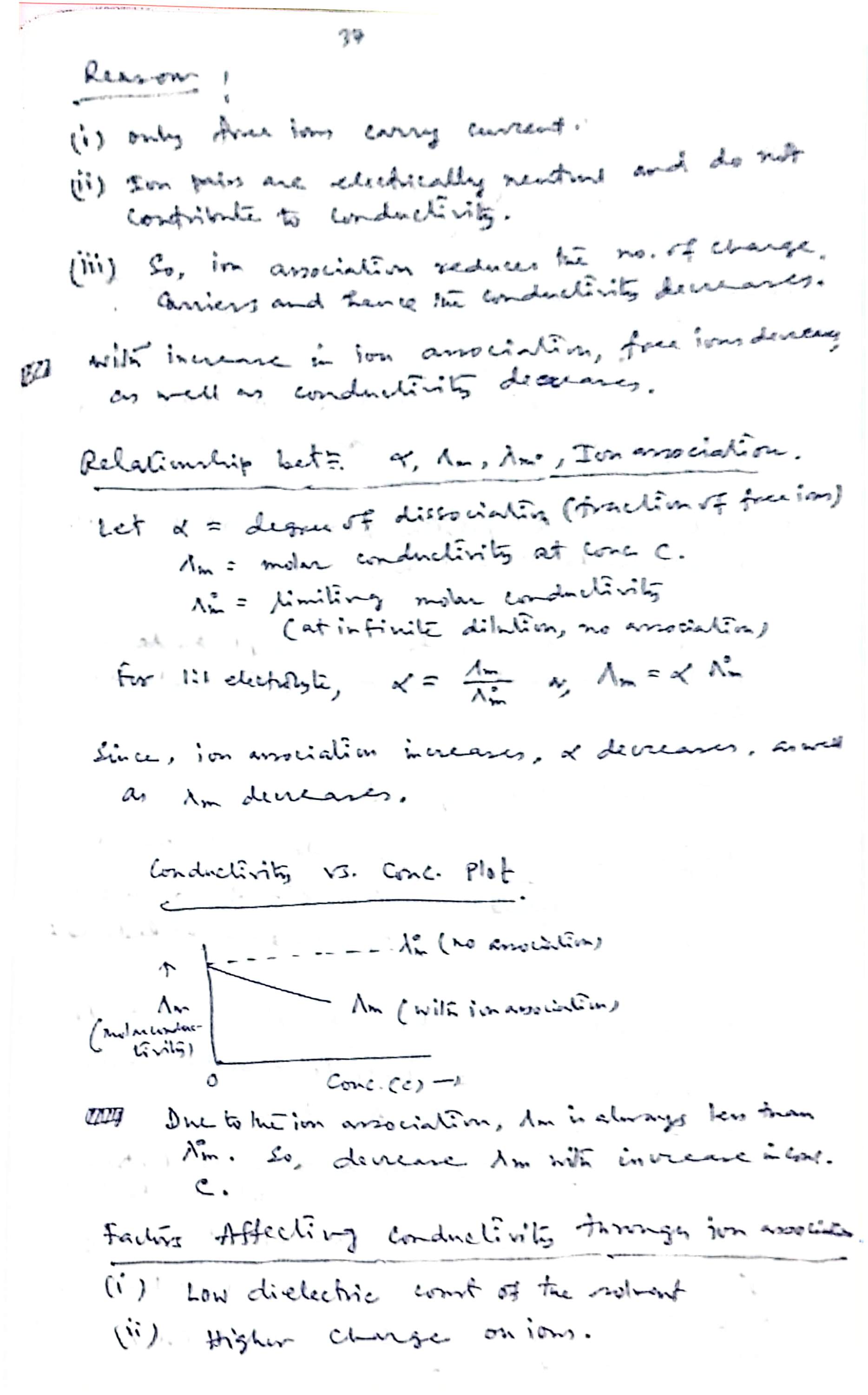
(i) Only free ions carry current. (ii) Ion pairs are electrically neutral and do not contribute to conductivity. (iii) So, ion association reduces the number of charge carriers — and hence the conductivity decreases. With increase in ion association, free ions decrease as well as conductivity decreases.

10 α, Λ(m), Λ(m)° — and the conductivity-vs-concentration plot

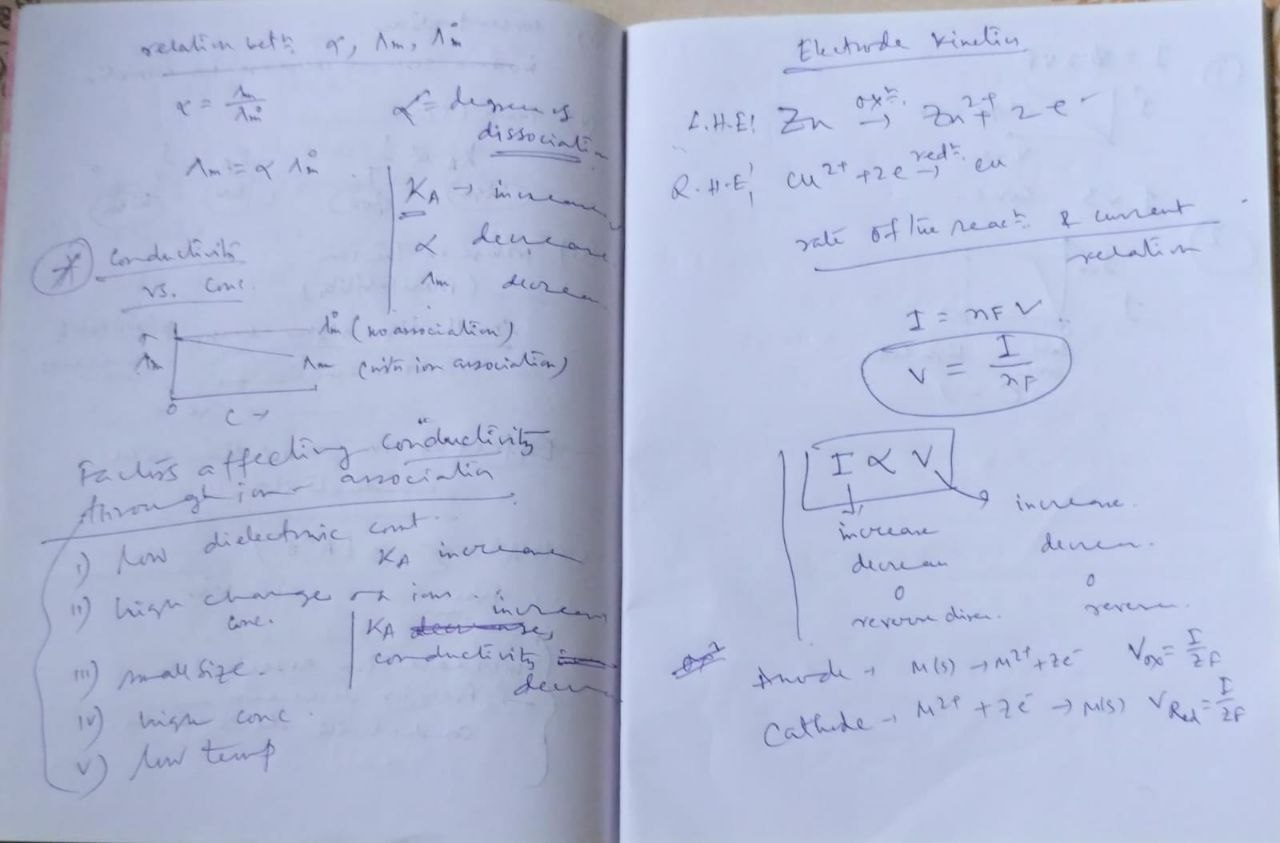
The notebook defines its three characters (p37):

$\alpha$ = degree of dissociation — the fraction of free ions;
$\Lambda_m$ = molar conductivity at concentration $c$ ;
$\Lambda_m^{\circ}$ = limiting molar conductivity (at infinite dilution, no association).

For a 1:1 electrolyte,

\alpha = \frac{\Lambda_m}{\Lambda_m^{\circ}} \qquad \text{or, equivalently,} \qquad \Lambda_m = \alpha\,\Lambda_m^{\circ}

Since ion association increases, $\alpha$ decreases — and so $\Lambda_m$ decreases. Because association is always present at finite concentration, $\Lambda_m$ is always less than $\Lambda_m^{\circ}$ , and the shortfall grows with $c$ . The notebook's plot draws Λ° as the dashed "no association" reference and Λm as the falling "with ion association" curve:

Fig 7. The notebook's conductivity-vs-concentration plot: dashed Λ(m)° (no association) above the falling Λ(m) (with association); the widening gap is (1−α)·Λ(m)° (Section 10, p37).

Consistency check with Class 3

Class 3 wrote the pair fraction as $\alpha_{\text{pair}} = 1 - \Lambda_c/\Lambda_c^{\circ}$ . Both statements are the same sentence from opposite sides: the notebook's $\alpha$ here is the free-ion fraction (degree of dissociation), so $\alpha_{\text{pair}} = 1 - \alpha$ . Keep track of which α a formula means — this is the same footing discipline as the N_A callout in Class 2.

11 Factors affecting conductivity — rerouted through association

Because conductivity is hostage to association, every factor of Sections 2–6 reappears as a conductivity factor with its arrow reversed. The notebook lists them (p37–38):

Low dielectric constant of the solvent → $K_A$ up → conductivity down.
Higher charge on ions → $K_A$ up → conductivity down.
Smaller size of ions → $K_A$ up → conductivity down.
Higher concentration → $K_A$ 's effect up → conductivity down.
Lower temperature → $K_A$ up → conductivity down.

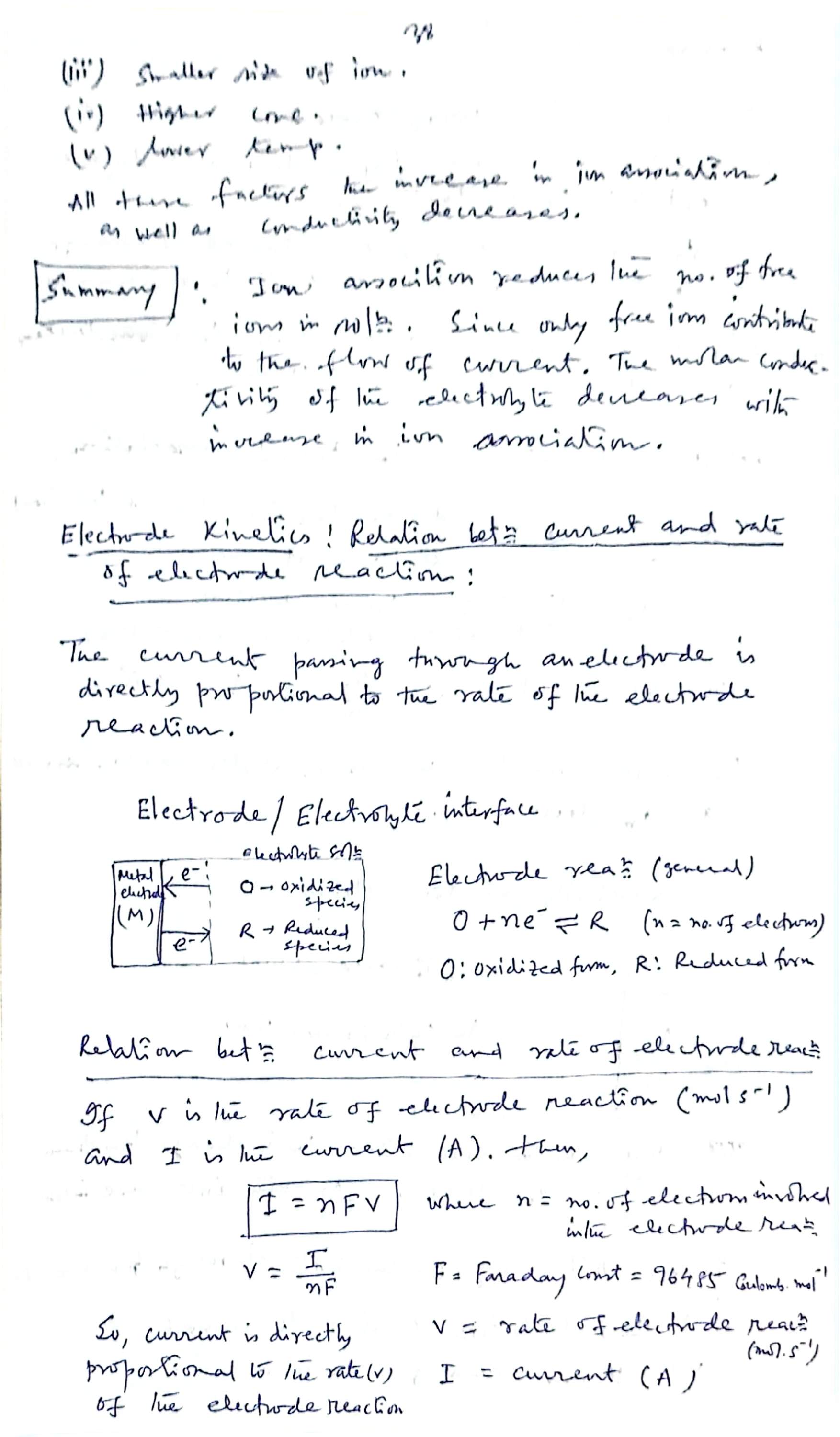
"All these factors increase in ion association, as well as conductivity decreases." The page-38 summary box closes the movement: ion association reduces the number of free ions in solution; since only free ions contribute to the flow of current, the molar conductivity of the electrolyte decreases with increase in ion association.

12 Electrode kinetics — the electrode/electrolyte interface

New topic, same lecture: the relation between current and the rate of an electrode reaction. The headline sentence of page 38 — the current passing through an electrode is directly proportional to the rate of the electrode reaction — is the whole section in one line; the rest is bookkeeping.

At the interface between a metal electrode (M) and the electrolyte solution, the oxidised species O and the reduced species R interconvert by exchanging electrons with the metal. The general electrode reaction:

\mathrm{O} + n\,e^- \rightleftharpoons \mathrm{R} \qquad (n = \text{no. of electrons})

Fig 8. The electrode/electrolyte interface: metal M | solution with oxidised O and reduced species interconverting via O + n e⁻ ⇌ R; electron direction chooses oxidation or reduction (Section 12, p38).

Read the double arrow literally: run electrons into the solution side and O is reduced to R; pull them out and R is oxidised to O. Which direction happens is a choice of the external circuit — and the rate of either direction is what the ammeter reads.

13 Current ↔ rate: the boxed relation

If $v$ is the rate of the electrode reaction (mol s⁻¹) and $I$ the current (A), then — boxed on page 38 —

vii

I = n F v

viii

v = \frac{I}{nF} \qquad \text{so } v \propto I

where $n$ = number of electrons involved in the electrode reaction and $F$ = Faraday constant = 96 485 coulombs mol⁻¹. The notebook then tabulates what the proportionality means operationally:

If current, I …	then rate of reaction, v …
increases	increases
decreases	decreases
is zero	is zero
reverses direction	reverses direction (oxidation ⇄ reduction swap)

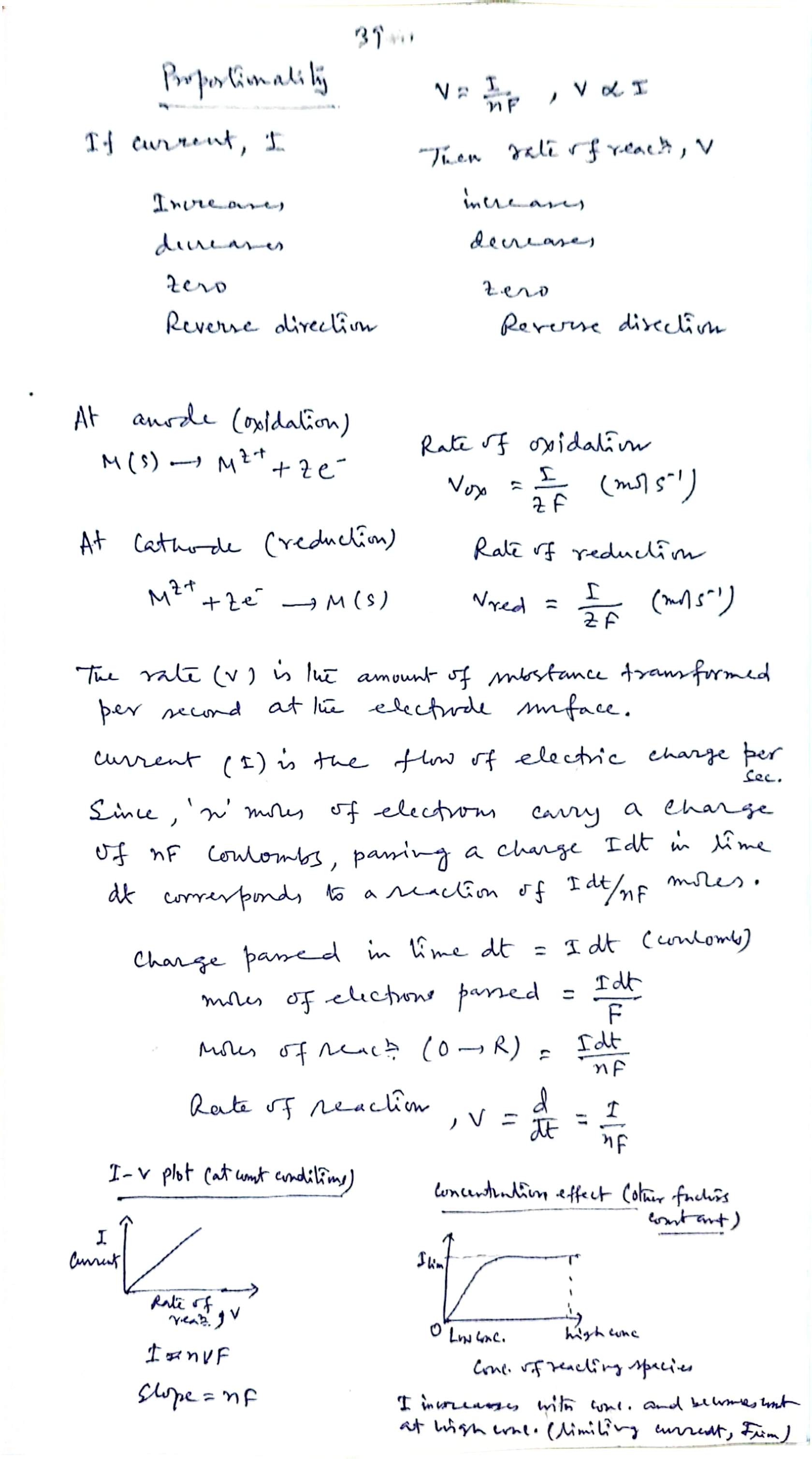
Where the box comes from (charge bookkeeping, p39)

The rate $v$ is the amount of substance transformed per second at the electrode surface; the current $I$ is the flow of electric charge per second. Since $n$ moles of electrons carry a charge of $nF$ coulombs, passing a charge $I\,dt$ in time $dt$ corresponds to a reaction of $I\,dt/nF$ moles:

Q = I\,dt \;\Rightarrow\; n_{e^-} = \frac{I\,dt}{F} \;\Rightarrow\; n_{\text{rxn}} = \frac{I\,dt}{nF} \;\Rightarrow\; v = \frac{dn_{\text{rxn}}}{dt} = \frac{I}{nF}

So, current is directly proportional to the rate of the electrode reaction — the ammeter is a rate meter.

visual lab 11

Current is a rate meter

Push current through the interface and watch O turn into R (or R into O when you reverse the leads). Electrons drift along the wire at a speed set by I; species convert one at a time at the electrode. The readouts below are the lecture's boxed relation evaluated exactly: v = I/(nF).

Current I — 5.0 mA

Electrons n

v = I/(nF) = 2.59 × 10⁻8 mol/s in 60 s: 1.55 × 10⁻6 mol, charge 0.3 C current forward ⇒ reaction runs O → R

Illustrates Sections 12–14: I = nFv with F = 96 485 C mol⁻¹; zero current means zero rate, and reversing the current reverses the reaction direction (the notebook's four-row proportionality table, p39). Dot speed and conversion tempo are an illustrative tempo only — the readouts evaluate the boxed equation exactly. Under reduced motion the stage renders static while the readouts stay live.

14 Rates at the anode and the cathode

For a metal electrode dissolving and depositing with $n = 2$ , the notebook writes both half-rates:

Electrode	Reaction	Rate
Anode (oxidation)	$\mathrm{M(s)} \rightarrow \mathrm{M}^{2+} + 2e^-$	$v_{ox} = \dfrac{I}{2F}$ (mol s⁻¹)
Cathode (reduction)	$\mathrm{M}^{2+} + 2e^- \rightarrow \mathrm{M(s)}$	$v_{red} = \dfrac{I}{2F}$ (mol s⁻¹)

From the in-class photo: a worked cell

The rough copy illustrates the pair on a familiar cell — left-hand electrode (L.H.E., anode): $\mathrm{Zn} \rightarrow \mathrm{Zn}^{2+} + 2e^-$ (oxidation); right-hand electrode (R.H.E., cathode): $\mathrm{Cu}^{2+} + 2e^- \rightarrow \mathrm{Cu}$ (reduction). At a current $I$ , both half-rates equal $I/2F$ : the same electrons that leave zinc enter copper, so the rate of zinc dissolving equals the rate of copper depositing. One current, two rates, one number.

15 The I–v line and the limiting current

Two plots close the lecture (p39). Left: at constant concentration, $I$ against $v$ is a straight line through the origin — $I = nFv$ — with slope $= nF$ . Right: with other factors fixed, $I$ against the concentration of the reacting species rises and then saturates at the limiting current $I_{lim}$ : "I increases with conc. and becomes constant at high conc."

Fig 9. A: I vs v is a straight line through the origin with slope nF (constant concentration). B: I vs concentration saturates at the limiting current I(lim) (Section 15, p39).

Why a plateau is honest physics

The current cannot exceed the rate at which O can reach the interface: once every arriving O is converted on arrival, pushing harder changes nothing — the reaction is supply-limited and $I$ flattens at $I_{lim}$ . The lecture states the observation; the reason is the same diffusion supply line that makes Class 2's mobility picture concentration-dependent.

16 Play with I = nFv

The lecture's boxed relation and its charge bookkeeping, live: set the current, the electron count and the time — the panel returns the charge, the moles of electrons, the moles reacted, the reaction rate and (with a molar mass) the mass transformed at the interface.

Current I (A)

Electrons n

Time t (s)

Molar mass M (g/mol)

Charge Q = I t

300.0 C

moles e⁻ = Q/F

3.11 × 10⁻3 mol

moles reacted = Q/(nF)

1.55 × 10⁻3 mol

rate v = I/(nF)

2.59 × 10⁻6 mol/s

mass transformed

0.102 g

Checks against the worked examples: 0.50 A, n = 2 → v = 2.59 × 10⁻⁶ mol/s and 600 s transforms 1.55 × 10⁻³ mol; 1.00 A for 1800 s with n = 2 → 9.33 × 10⁻³ mol, i.e. 0.610 g of Zn (M = 65.38) dissolved or 0.593 g of Cu (M = 63.55) deposited. F = 96 485 C mol⁻¹ throughout.

17 The equation sheet, at a glance

Every boxed or underlined result of the lecture on one screen; labels match the sections above.

K_A \propto \frac{1}{\varepsilon_r}

iii

K_A \propto |z_+\,z_-|

K_A \propto \frac{1}{T}

\alpha = \frac{\Lambda_m}{\Lambda_m^{\circ}} \;\Longleftrightarrow\; \Lambda_m = \alpha\,\Lambda_m^{\circ}

vii

I = n F v

viii

v = \frac{I}{nF}

v_{ox} = \frac{I}{2F}, \qquad v_{red} = \frac{I}{2F}

n_{\text{rxn}} = \frac{I\,t}{nF}, \qquad Q = I\,t

18 Symbol table

Symbol	Meaning	Typical unit
$K_A$	Association constant (Bjerrum, Class 3); extent of ion-pair formation	mol⁻¹ L
$\varepsilon_r$	Relative permittivity (dielectric constant) of the solvent	dimensionless (water ≈ 78, 298 K)
$z_+, z_-$	Charge numbers of cation and anion	dimensionless
$c$	Molar concentration of the electrolyte	mol L⁻¹
$T$	Absolute temperature	K
$\alpha$	Degree of dissociation — free-ion fraction, $0 \le \alpha \le 1$ (this lecture's convention)	dimensionless
$\Lambda_m, \Lambda_m^{\circ}$	Molar conductivity at $c$ ; limiting molar conductivity (no association)	S cm² mol⁻¹
$I$	Current through the electrode	A (= C s⁻¹)
$v$	Rate of the electrode reaction (substance transformed per second at the interface)	mol s⁻¹
$v_{ox}, v_{red}$	Rate of oxidation (anode); rate of reduction (cathode)	mol s⁻¹
$n$	Number of electrons in the electrode reaction	dimensionless
$F$	Faraday constant, charge per mole of electrons	96 485 C mol⁻¹
$Q$	Charge passed, $Q = I t$	C
$t$	Time of electrolysis	s
$I_{lim}$	Limiting current — supply-saturated plateau at high concentration	A
O, R	Oxidised / reduced species of the general electrode reaction	—

19 Rapid revision — 14 lines before the exam

Ion-pair equilibrium: $\mathrm{A}^{2+} + \mathrm{B}^{2-} \rightleftharpoons \mathrm{AB}$ ; the six factors are statements about $K_A$ .
Solvent: $K_A \propto 1/\varepsilon_r$ — low ε(r) (nitrobenzene) pairs, high ε(r) (water) solvates and separates.
Charge: $K_A \propto |z_+z_-|$ — ladder 1 (KCl, least) → 2 (CaCl₂) → 4 (MgSO₄) → 6 (Al₂(SO₄)₃, maximum).
Size: smaller ion → higher charge density → closer approach → more association; Li⁺ > Na⁺ > K⁺ > Rb⁺ > Cs⁺ and F⁻ > Cl⁻ > Br⁻ > I⁻ in association.
Concentration: higher c → ions closer → pair probability up. Temperature: $K_A \propto 1/T$ — cold pairs, hot separates.
Polarizing power (higher charge, smaller size) distorts the partner's solvent sheath → stronger attraction → more association.
Conductivity bill: only free ions carry current; ion pairs are neutral ⇒ association ↑ → carriers ↓ → conductivity ↓.
$\alpha = \Lambda_m/\Lambda_m^{\circ}$ (free-ion fraction, 1:1); $\Lambda_m = \alpha\Lambda_m^{\circ}$ ; Λ(m) always < Λ(m)° at finite c.
Conductivity factors = association factors with arrows reversed: low ε(r), high charge, small size, high conc., low temp.
Electrode kinetics headline: current ∝ rate of electrode reaction; general reaction O + n e⁻ ⇌ R at the metal/solution interface.
Boxed: $I = nFv$ ; equivalently $v = I/(nF)$ ; F = 96 485 C mol⁻¹; I = 0 ⇒ v = 0; reverse I ⇒ reverse reaction direction.
Bookkeeping: charge in dt = I dt; moles e⁻ = I dt/F; moles reacted = I dt/(nF) ⇒ v = I/(nF).
Anode M → M²⁺ + 2e⁻ and cathode M²⁺ + 2e⁻ → M both run at I/2F; Zn/Cu cell: same current, same rate both sides.
I–v plot: straight line through origin, slope nF. I vs conc.: rises then plateaus at the limiting current I(lim).

Next up: Class 5 is live — exchange current, overpotential, the Butler–Volmer equation and the Tafel line.

Read Class 5 →

20 Original notebook scans

Digitised from the class notebook of 05 Sep 2026 — notebook pages 34–39 (CamScanner spreads S1–S6, the fair copy) plus the three in-class phone photos N1–N3; every equation above was cross-checked against these pages. Tap any thumbnail to open the full scan.

N1 · 5/9/26 header, factor 1 (solvent, εr)

N2 · factors 2–6, conductivity effect

N3 · α–Λ(m) relation, Λ vs c plot, Zn/Cu electrode kinetics

S1 · p34 · factors 1–2, εr boxes, charge table

S2 · p35 · size series, concentration, temperature

S3 · p36 · polarizing power, summary, carriers before/after

S4 · p37 · reasons, α = Λ(m)/Λ(m)°, Λ vs c plot

S5 · p38 · conductivity summary, interface, boxed I = nFv

S6 · p39 · proportionality table, anode/cathode rates, I–v & I(lim)

21 PYQ bank · University papers 2020–2024

Same audit as Classes 1–3: every page of the five M.Sc. Semester-I question papers (2020–2024 — all subjects MSCH-101…106, 60 scanned pages) OCR'd and verified by hand; the Physical Chemistry paper each year is MSCH-104 (Physical General-I). The rule is unchanged: only questions that actually appeared, tagged with year and repeat count.

Year	Physical paper (MSCH-104)	Pages verified	Class-4 questions (association factors / conductivity cost / electrode kinetics)
2020	Physical General I (new + old syllabus copies)	p. 12–15	0 — group theory, QM, stat-thermo, rotational/vibrational spectroscopy, fullerenes
2021	Physical General I (+ internal)	p. 7–8	0 — group theory, QM, partition functions, nanotubes, Raman
2022	Physical General I	p. 9–10	0 — symmetry, operators, spectroscopy, stat-thermo
2023	Physical General I	p. 9–10	0 — point groups, operators, rotors, Raman, fullerenes, stat-thermo
2024	Physical General I	p. 12–13	0 — group theory, matrices, rotors, polarizability, partition functions

Honest verdict

Across 2020–2024 the university never asked an association-factors, conductivity-of-association or electrode-kinetics question in these papers — MSCH-104 in those years is entirely group theory, quantum mechanics, spectroscopy and statistical thermodynamics — so, per the rule, the year-tagged bank stays empty rather than being padded with look-alikes. The moment one appears it lands here with its year and repeat count. For practice, four worked examples in the lecture's own style are answered in full below.

Worked examples — the lecture's equations, exercised

Ex. 1electrode kinetics · I = nFvSection 13

Q. A current of 0.50 A drives a two-electron electrode reaction ( $n = 2$ ). Find the rate of the electrode reaction, and the amount transformed in 10 minutes.

Ans. $v = I/(nF) = 0.50/(2 \times 96\,485) = 2.59 \times 10^{-6}$ mol s⁻¹. In $t = 600$ s: $n_{\text{rxn}} = v t = 2.59 \times 10^{-6} \times 600 = 1.55 \times 10^{-3}$ mol (equivalently $Q = It = 300$ C and $n_{\text{rxn}} = Q/2F$ ). A wristwatch current already moves micromoles — which is why coulometry is a practical analytical method.

Ex. 2anode rate · Zn/Cu cellSection 14

Q. In the Zn | Zn²⁺ ‖ Cu² | Cu cell of the in-class photo, a current of 1.00 A is passed for 30 minutes. How much zinc dissolves at the anode, and how much copper deposits at the cathode? (M(Zn) = 65.38 g mol⁻¹, M(Cu) = 63.55 g mol⁻¹.)

Ans. Both half-rates equal $I/2F = 1.00/192\,970 = 5.18 \times 10^{-6}$ mol s⁻¹. In 1800 s: $n = 9.33 \times 10^{-3}$ mol on each electrode. Masses: Zn dissolved $= 9.33 \times 10^{-3} \times 65.38 = 0.610$ g; Cu deposited $= 9.33 \times 10^{-3} \times 63.55 = 0.593$ g. Same moles, different masses — one current, two rates, one number.

Ex. 3α from conductivitySection 10

Q. A 1:1 electrolyte shows $\Lambda_m = 120$ S cm² mol⁻¹ at a concentration where $\Lambda_m^{\circ} = 150$ S cm² mol⁻¹. What fraction of the ions is free, and what fraction is associated?

Ans. $\alpha = \Lambda_m/\Lambda_m^{\circ} = 120/150 = 0.80$ : 80 % free ions, so the associated (paired, non-conducting) fraction is $1 - \alpha = 0.20$ , i.e. 20 %. The conductivity gap $(1-\alpha)\Lambda_m^{\circ} = 30$ S cm² mol⁻¹ is precisely the current the ion pairs refused to carry.

Ex. 4factor arrows · reasoningSections 2–8

Q. Predict and justify: (a) which of KCl, MgSO₄, Al₂(SO₄) associates most; (b) what happens to the molar conductivity of MgSO₄ when the solution is (i) diluted, (ii) heated.

Ans. (a) $|z_+z_-|$ : KCl = 1, MgSO₄ = 4, Al₂(SO₄)₃ = 6 ⇒ Al₂(SO₄)₃ associates most ( $K_A \propto |z_+z_-|$ ). (b)(i) Dilution lowers the paired fraction (α → 1 as c → 0), so more carriers ⇒ $\Lambda_m$ rises towards $\Lambda_m^{\circ}$ . (ii) Heating lowers $K_A$ ( $K_A \propto 1/T$ ), pairs dissociate, carriers increase ⇒ $\Lambda_m$ increases (association component; the viscosity-driven mobility rise of Class 2 adds in the same direction).